In This Topic
Model
Minitab calculates K – 1 logit functions for a model with K response categories. For example, a response with three categories (1, 2, 3) has two logit functions (reference event = 3):
Formula
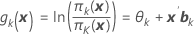
Notation
| Term | Description |
|---|---|
| gk ( x ) | logit link function |
| θk | constant associated with the k th distinct response category |
| x k | vector of predictor variables |
| b k | vector of coefficients associated with the k th logit function |
Factor/covariate pattern
Describes a single set of factor/covariate values in a data set. Minitab calculates event probabilities, residuals, and other diagnostic measures for each factor/covariate pattern.
For example, if a data set includes the factors gender and race and the covariate age, the combination of these predictors may contain as many different covariate patterns as subjects. If a data set only includes the factors race and sex, each coded at two levels, there are only four possible factor/covariate patterns. If you enter your data as frequencies, or as successes, trials, or failures, each row contains one factor/covariate pattern.
Event probability
Denoted as π. For a three-category model with categories 1, 2, and 3 (reference event 3), the conditional probabilities are:
Formula
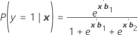
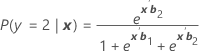
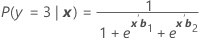
And the event probability is:
π k (x) = P(y = k| x ) for k = 1, 2, 3. Each probability is a function of the vector of 2(p + 1) parameters, b ' = ( b '1, b '2)
Log-likelihood
The log-likelihood function is maximized to yield optimal values of b. For a model with 3 response categories (reference = 3), the log-likelihood function is:

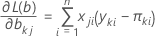
The maximum likelihood estimates are obtained by setting these equations to zero and solving for b.
Notation
| Term | Description |
|---|---|
| k | 1, 2 |
| j | 0, 1, 2, ..., p |
| p | number of coefficients in the model, not including the constant coefficients |
| πki | πk(xi), with x0i for each subject |
Coefficients
The maximum likelihood estimates, also called parameter estimates. If there are K distinct response values, Minitab estimates K – 1 sets of parameter estimates for each predictor. The effects vary according to the response category compared to the reference event. Each logit provides the estimated differences in the log odds of one response category versus the reference event. Parameters in the K – 1 equations determine parameters for logits using all other pairs of response categories.
The estimated coefficients are calculated using an iterative reweighted least squares method, which is equivalent to maximum likelihood estimation.1,2
References
- D.W. Hosmer and S. Lemeshow (2000). Applied Logistic Regression. 2nd ed. John Wiley & Sons, Inc.
- P. McCullagh and J.A. Nelder (1992). Generalized Linear Model. Chapman & Hall.
Standard error of coefficients
Asymptotic standard error, which indicates the precision of the estimated coefficient. The smaller the standard error, the more precise the estimate.
See [1] and [2] for more information.
- A. Agresti (1990). Categorical Data Analysis. John Wiley & Sons, Inc.
- P. McCullagh and J.A. Nelder (1992). Generalized Linear Model. Chapman & Hall.
Z
Z is used to determine whether the predictor is significantly related to the response. Larger absolute values of Z indicate a significant relationship. The p-value indicates where Z falls on the normal distribution.
Formula
Z = βi / standard error
The formula for the constant is:
Z = θk / standard error
For small samples, the likelihood-ratio test may be a more reliable test of significance.
p-value (P)
Used in hypothesis tests to help you decide whether to reject or fail to reject a null hypothesis. The p-value is the probability of obtaining a test statistic that is at least as extreme as the actual calculated value, if the null hypothesis is true. A commonly used cut-off value for the p-value is 0.05. For example, if the calculated p-value of a test statistic is less than 0.05, you reject the null hypothesis.
Odds ratio
Useful in interpreting the relationship between a predictor and response.
The odds ratio (q) can be any nonnegative number. An odds ratio of 1 serves as the baseline for comparison. If θ = 1, there is no association between the response and predictor. If θ > 1, the odds of the comparison response event are higher for the reference level of the factor (or for higher levels of a continuous predictor). If θ < 1, the odds of the comparison response event are less for the reference level of the factor (or for higher levels of a continuous predictor). Values farther from 1 represent stronger degrees of association.
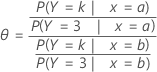
For example, for a model with three response categories (1, 2, 3) and one predictor, the odds ratio specifies the odds for outcome category k versus the outcome category used as the reference event (in this example, 3). The following is a formula for the odds ratio for a predictor with two levels, a and b.
Formula
Notation
| Term | Description |
|---|---|
| k | outcome category |
Confidence interval
Formula
The large sample confidence interval for βi is:
β i + Zα /2* (standard error)
To obtain the confidence interval of the odds ratio, exponentiate the lower and upper limits of the confidence interval. The interval provides the range in which the odds may fall for every unit change in the predictor.
Notation
| Term | Description |
|---|---|
| α | significance level |
Variance-covariance matrix
A square matrix with the dimensions p +1 × (K – 1). The variance of each coefficient is in the diagonal cell and the covariance of each pair of coefficients is in the appropriate off-diagonal cell. The variance is the standard error of the coefficient squared.
The variance-covariance matrix is asymptotic and is obtained from the final iteration of the inverse of the information matrix. The matrix of second partial derivatives are used to obtain the covariance matrix.
Notation
| Term | Description |
|---|---|
| p | number of predictors |
| K | number of categories in the response |
Pearson
A summary statistic based on the Pearson residuals that indicates how well the model fits your data. Pearson isn't useful when the number of distinct values of the covariate is approximately equal to the number of observations, but is useful when you have repeated observations at the same covariate level. Higher χ2 test statistics and lower p-values values indicate that the model may not fit the data well.
The formula is:

where r = Pearson residual, m = number of trials in the jth factor/covariate pattern, and π0 = hypothesized value for the proportion.
Deviance
A summary statistic based on the Deviance residuals that indicates how well the model fits your data. Deviance isn't useful when the number of distinct values of the covariate is approximately equal to the number of observations, but is useful when you have repeated observations at the same covariate level. Higher values of D and lower p-values values indicate that the model may not fit the data well. The degrees of freedom for the test is (k - 1)*J − (p) where k is the number categories in the response, J is the number of distinct factor/covariate patterns and p is the number of coefficients.
The formula is:
D =2 Σ yik log p ik− 2 Σ yik log π ik
where πik = probability of the ith observation for the kth category.