An agricultural engineer studies the effect of five factors on the growth of basil plants. The engineer designs a 2-level Taguchi experiment to determine which factor settings increase the plant's rate of growth without increasing the variability in growth. The engineer also manipulates two noise factors to determine which settings for the five factors increase plant growth across the true range of temperature and humidity conditions.
The engineer creates a dynamic design with a signal factor, Time, which is the amount of growth time at 4 levels (3, 5, 7, and 9). The engineer collects and records the data into four columns of the worksheet.
Choose Stat > DOE > Taguchi > Analyze Taguchi Design.
In Response data are in, enter T1H1, T1H2, T2H1, and T2H2.
Click Graphs, then under Generate plots of main effects and interactions in the
model for select Standard deviations. Click OK.
Click Analysis.
Under Display response tables for, check all options. Under Fit linear model for, check all options. Click OK.
Click Terms.
Move terms A: Variety, B: Light, C: Fertilizer, D: Water, E: Spraying, and AC from Available Terms to Selected Terms. Click OK.
Click Options.
Under Dynamic signal-to-noise ratio, select Fit all lines through a fixed reference
point.
Click OK in each dialog box.
Interpret the results
Minitab provides an estimated regression coefficients table for each response characteristic that you select. Use the p-values to determine which factors are statistically significant and use the coefficients to determine each factor's relative importance in the model.
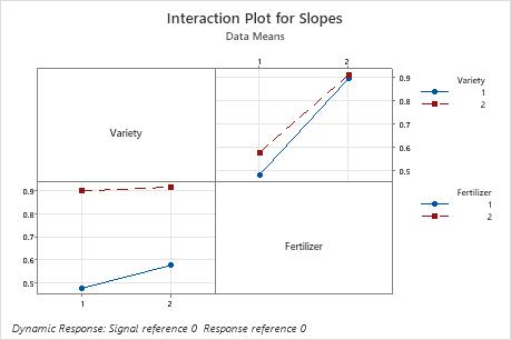
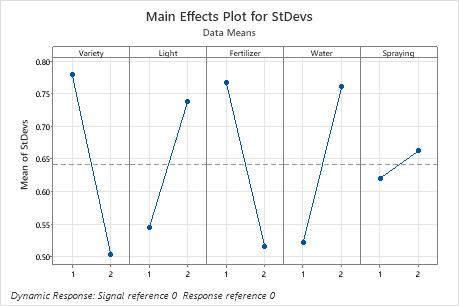
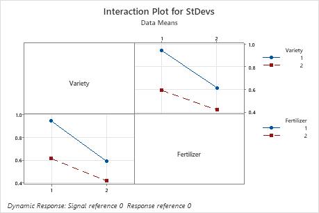
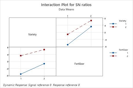
In this example, for S/N ratios, Fertilizer has a p-value less than 0.05 (p = 0.033) and is statistically significant at a significance level of 0.05. Variety is statistically significant at a significance level of 0.10 (p = 0.064). For the slopes, none of the factors are statistically significant at a significance level of 0.05 or 0.10. For the standard deviations, the p-values indicate that Variety (p = 0.050) is statistically significant at the 0.05 significance level. Fertilizer (p = 0.054), Water (p = 0.057), and Light (p = 0.070) are statistically significant at the 0.10 significance level. Spraying (p = 0.300) and the interaction, Fertilizer*Variety (p = 0.169) are not statistically significant.
The absolute value of the coefficient indicates the relative strength of each factor. The factor with the largest coefficient has the largest impact on a given response characteristic. In Taguchi designs, the magnitude of the factor coefficient usually mirrors the factor ranks in the response tables.
The response tables show the average of each response characteristic for each level of each factor. The tables include ranks based on Delta statistics, which compare the relative magnitude of effects. The Delta statistic is the highest minus the lowest average for each factor. Minitab assigns ranks based on Delta values; rank 1 to the highest Delta value, rank 2 to the second highest, and so on. Use the level averages in the response tables to determine which level of each factor provides the best result.
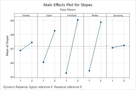
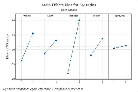
In dynamic Taguchi experiments, you always want to maximize the S/N ratio. In this example, the ranks indicate that Fertilizer has the most influence on both the S/N ratio and the slope. For S/N ratio, Variety has the next largest influence, followed by Water, Light, and Spraying. For slopes, Water has the next largest influence, followed by Light, Variety, and Spraying. For the standard deviations, the ranks are Variety, Fertilizer, Water, Light, and Spraying.
For this example, the engineer wants the factor levels that minimize the standard deviation and maximize the S/N ratio and the slope. The level averages in the response tables show that the S/N ratios and the slopes were maximized using these levels:
Variety, Level 2
Fertilizer, Level 2
Spraying, Level 2
There is not a consensus on the best levels for Light and Water, because S/N and slopes are maximized at level 2, but standard deviations are minimized at level 1.