Select the method or formula of your choice.
In This Topic
Coefficient (Coef)
Minitab uses least squares estimation to calculate the coefficients.
In matrix terms, the least squares estimates of the coefficients are:
b = (X'X)-1X'y
For more information on coefficients of higher order models, see Cornell1.
Notation
| Term | Description |
|---|---|
| X | design matrix |
| y | response column |
- J.A. Cornell (1990). Experiments With Mixtures: Designs, Models, and the Analysis of Mixture Data, John Wiley & Sons.
Standard error of the coefficient (SE Coef)
For simple linear regression, the standard error of the coefficient is:

The standard errors of the coefficients for multiple regression are the square roots of the diagonal elements of this matrix:

Notation
| Term | Description |
|---|---|
| xi | ith predictor value |
 | mean of the predictor |
| X | design matrix |
| X' | transpose of the design matrix |
| s2 | mean square error |
T-value

Notation
| Term | Description |
|---|---|
 | test statistic for the  coefficient coefficient |
 |  estimated coefficient estimated coefficient |
 | standard error of the  estimated coefficient estimated coefficient |
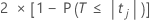
P-value – Coefficients table
The two-sided p-value for the null hypothesis that a regression coefficient equals 0 is:
The degrees of freedom are the degrees of freedom for error, as follows:
n – p
Notation
| Term | Description |
|---|---|
 | The cumulative distribution function of the t distribution with degrees of freedom equal to the degrees of freedom for error. |
| tj | The t statistic for the jth coefficient. |
| n | The number of observations in the data set. |
| p | The sum of the degrees of freedom for the terms. |
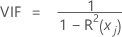
Variance inflation factor (VIF)
The VIF can be obtained by regressing each predictor on the remaining predictors and noting the R2value.
Formula
For predictor xj, the VIF is:
Notation
| Term | Description |
|---|---|
| R2( xj) | coefficient of determination with xj as the response variable and the other terms in the model as the predictors |