A textile manufacturer developed a solar energy system to pre-heat feed water for a boiler that is part of the power system for the manufacturing process. A technician monitors the amount of energy that is used each hour to make sure that the pre-heat process is stable.
After confirming that the data is stable and does not include any outliers, the technician conducts a normality test and finds that the data does not follow a normal distribution. The technician then conducts a Box-Cox analysis to determine whether a Box-Cox transformation is appropriate before creating an I-MR chart of the data.
- Open the sample data, SolarEnergyProcess.MWX.
- Choose .
- In All observations for a chart are in one column, enter Energy.
- In Subgroup sizes, enter 1.
- Click OK.
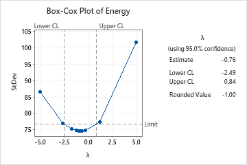
Interpret the results
For the Box-Cox transformation, a λ value of 1 is equivalent to using the original data. Therefore, if the confidence interval for the optimal λ includes 1, then no transformation is necessary. In this example, the 95% confidence interval for λ (−2.49 to 0.84) does not include 1, so a transformation is appropriate. The estimated value for the optimal λ is −0.76. Because the rounded value of −1 is within the confidence interval, the technician should transform the data using λ = −1. A transformation that uses λ = −1 corresponds to the inverse transformation (transformed value = 1 / original value).