Download the Macro
Be sure that Minitab knows where to find your downloaded macro. Choose . Under Macro location browse to the location where you save macro files.
Important
If you use an older web browser, when you click the Download button, the file may open in Quicktime, which shares the .mac file extension with Minitab macros. To save the macro, right-click the Download button and choose Save target as.
Required Inputs
You need one column of time series data.
Optional Inputs
- AR K…K
- If you have any estimated auto-regressive parameters and you want to execute spectral model checking, enter these parameters here.
- DIF K
- If you have a differencing component, enter the differencing order here.
- MA K…K
- If you have any estimated moving average parameters and you want to execute spectral model checking, enter these parameters here.
- VARIANCE K
- Enter your estimated variance (default = 1.0).
- SMOOTH K
- Enter the length of the moving average (default = 3). The length of the moving average must be an odd integer.
- ONEDOC
- Enter if you want all graphs on one page.
- SPERIOD C C
- Enter if you want to store the coordinates for the periodogram. The first column will contain I(omega) and the second column will contain omega.
- SCUMUL C C C C
- Enter if you want to store the coordinates for the cumulative periodogram. The first column will contain U(j), the second column will contain the upper significance limit, the third column will contain the lower significance limit, and the fourth column will contain the X-axis.
- SSPEC C C C C
- Enter if you want to store the coordinates for the spectral estimate. The first column will contain the spectral estimate, the second column will contain the upper confidence limit, the third column will contain the lower confidence limit, and the fourth column will contain omega.
- SMODEL C C C C
- Enter if you want to store the coordinates for the spectral model check. The first column will contain F(omega), the second column will contain the upper confidence limit, the third column will contain the lower confidence limit, the fourth column will contain the spectral estimates, and the fifth column will contain omega.
Running the Macro
Suppose the data are in C1. To run the macro, choose and type:
%SPECTRAL C1Click Run.
Additional Information
Periodogram
The periodogram is a tool that can be used to detect cyclical components in a time series. The periodogram is defined as follows:
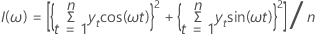

While the periodogram is defined for ω = 0, this point is excluded because it corresponds to the sample mean (which is of no interest). If n is odd, we exclude ω =π.
Cumulative Periodogram
The cumulative periodogram is a direct application of the periodogram for testing the hypothesis that a particular time series is a white noise sequence. The cumulative periodogram is an effective diagnostic tool for residuals. The cumulative periodogram is defined as:
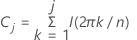
j=1,...,m where m is the largest integer strictly less than n/2

A plot of U j against j /(m −1) is known as the cumulative periodogram.
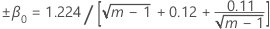
We can also define critical values for testing the white noise hypothesis. The level of significance that the macro uses is 10% (critical value = 1.224). Two parallel lines with the following y-intercept define the critical region:
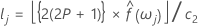
Spectral Estimate
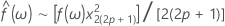
The spectral estimate,  ,
can be derived by simply taking a moving average of order 2p+1 (where p is a
positive integer) of the ordinates calculated by the periodogram. We can also
set confidence limits on this spectral estimate:
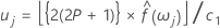
,
can be derived by simply taking a moving average of order 2p+1 (where p is a
positive integer) of the ordinates calculated by the periodogram. We can also
set confidence limits on this spectral estimate:
The upper and lower confidence limits can be defined as:
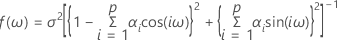
Spectrum of an ARMA Process
The spectral estimate is the estimate of the spectrum based on the data. The spectrum is based on the true population values for the model parameters. The spectrum of an AR(p) process can be defined as follows:
The spectrum of a MA(q) process can be defined as follows:
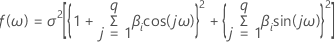
The spectrum of an ARMA (p, q) (where p and q are orders) process can be defined as follows:

Spectral Model Checking for an ARIMA Process
We can compare the spectral estimate computed from an observed time series to the true spectrum based on the model parameters. Intuitively, if the spectral estimate is approximately statistically equal to the true spectrum we can conclude that our estimated model parameters are adequate in modeling the series.


Thus, we can set confidence limits to determine whether or not the spectral estimate lies within these limits.
Example 1
For an example of the periodogram, cumulative periodogram, and spectral estimate, consider the data set 'Cycle 1, late follicular phase' (Diggle, p. 228). To run the macro, choose and type:
%SPECTRAL C1First, the periodogram (not shown) indicates that this series does have a cyclical component to it because of its dominant peak. Sometimes, the X-axis is transformed to a more meaningful scale so that it can be more easily determined at which point in time the cyclical component is occurring. For this reason, the macro has storage options so that the user may transform the axis (you may then use the graphics capabilities in MINITAB to generate plots). Second, the cumulative periodogram indicates that this series is not a white noise sequence because some of the data points go beyond the significance limits (represented by the parallel dotted lines). Finally, the spectral estimate (computed by the default 3-point moving average) is displayed by the red line while the confidence limits are displayed by the dotted lines. This plot gives us some sense about what the true population spectrum may look like. All three plots match the plots given in Diggle (p. 52, 55, 106).
Example 2
For a complete ARIMA analysis, consider the data set, 'Cycle 2, early follicular phase' (Diggle, p. 228). First, compute the periodogram, the cumulative periodogram, and the spectral estimate. I will also place these three plots on one page using the 'Onedoc' subcommand. Choose and type:
%SPECTRAL C2;
ONEDOC.
The graphs (not shown), make it clear that this time series is not a white noise sequence because both the periodogram and the spectral estimate indicate a low frequency series because of the dominant peaks at small values of omega, and the cumulative periodogram displays significant points. Thus, we will use MINITAB to model this time series using the ARIMA algorithm. After looking at various models, the best one is an AR(1).
Now, we will use the macro to evaluate this empirical model. Notice how the estimate of the auto-regressive parameter and the estimate of the variance (from the ARIMA output) are entered in the following command language. Choose and type:
%SPECTRAL C2;
AR 0.5860;
VARIANCE 0.20603;
ONEDOC.
The resulting plots simply redisplay the graphs already seen along with the spectral model check. In reference to the spectral model check, the red circles represent the spectral estimate, and the black solid line is the 'true' spectrum based on our estimated ARIMA model parameters. The dotted lines represent the confidence limits for the 'true' spectrum. Since almost all of the three point moving averages (red circles) are contained within the confidence interval for the true spectrum, we can conclude that the model is valid. Lastly, we would want to execute the macro on the residuals to make sure they are white noise residuals. The cumulative periodogram does, in fact, indicate that the residuals follow a white noise sequence.
References
Diggle, P. J. Time Series, A Biostatistical Introduction. Oxford: Clarendon Press, 1990.