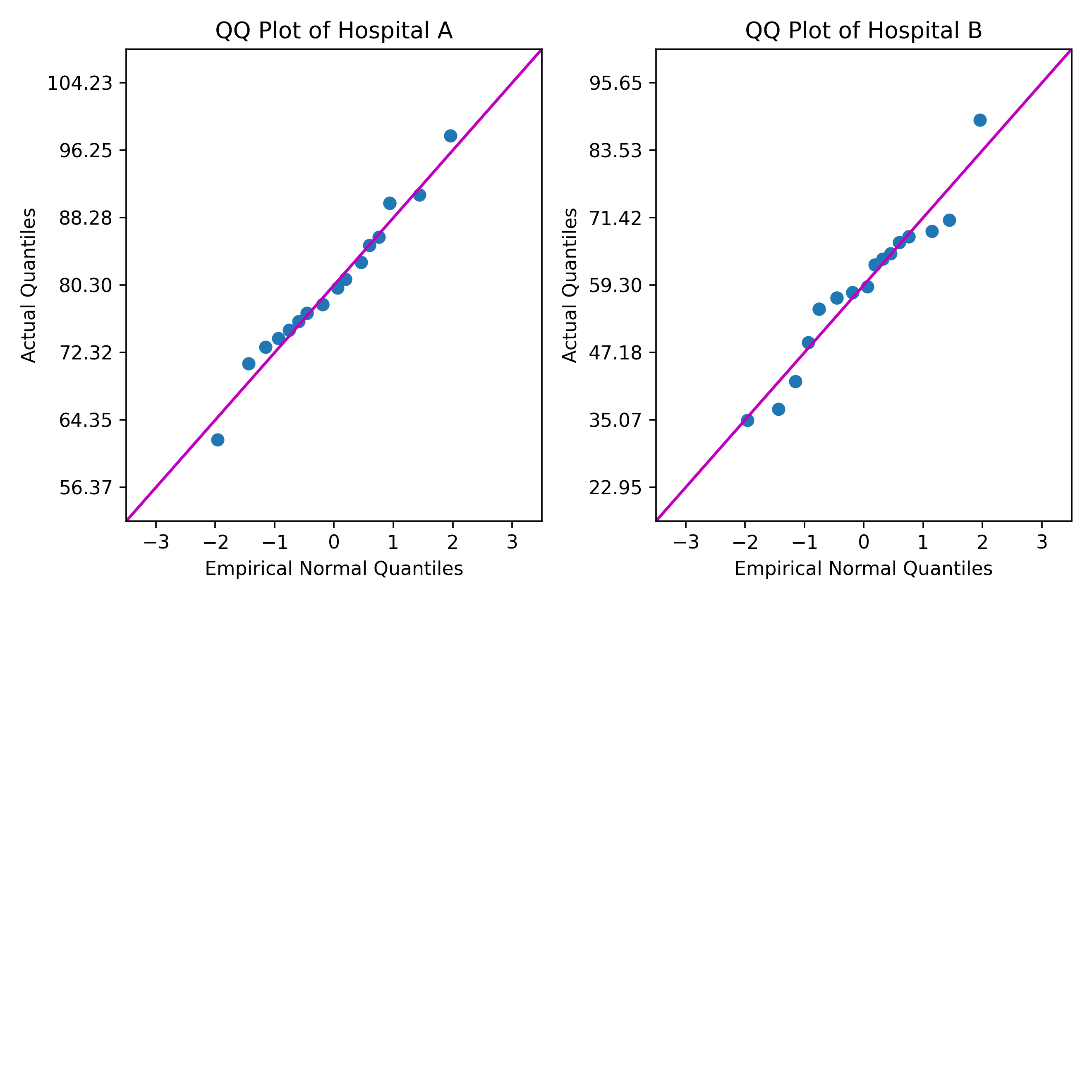
Un consultor de atención médica desea comparar la normalidad de las calificaciones de satisfacción de los pacientes de dos hospitales utilizando una gráfica de cuantiles-cuantiles (QQ). Las gráficas QQ muestran qué tan bien se ajusta cada conjunto de calificaciones de satisfacción de los pacientes a una distribución normal.
El script de ejemplo de Python lee los datos de las columnas de Minitab. El script calcula los cuantiles y crea una gráfica QQ para cada columna. Luego, el script envía las gráficas a la sección Salida de Minitab.
Todos los archivos a los que se hace referencia en esta guía están disponibles en este archivo .ZIP: python_guide_files.zip.
Utilice los siguientes archivos para llevar a cabo los pasos de esta sección:
| Archivo | Descripción |
|---|---|
| qq_plot.py | Un script de Python que toma columnas de una hoja de trabajo de Minitab y muestra la gráfica QQ para cada columna. |
Para el script de Python del ejemplo siguiente se requieren los siguientes módulos de Python. El número entre paréntesis es la versión más reciente del paquete que usamos para ejecutar el script.
- mtbpy
- El módulo de Python que integra Minitab y Python. En el ejemplo, las funciones de este módulo envían los resultados de Python a Minitab.
- numpy (1.24.2)
- Un módulo de Python que tiene varias aplicaciones para cálculos científicos y numéricos.
- matplotlib (3.7.0)
- Un módulo de Python que tiene varias funciones relacionadas con el trazado de gráficas y la creación de figuras.
- Asegúrese de haber instalado los módulos necesarios: mtbpy y numpy.
- Para instalar los módulos necesarios por medio de PIP, ejecute el comando correspondiente para el terminal de su sistema operativo (por ejemplo, el Microsoft® Windows Command Prompt o el Terminal macOS):
pip install mtbpy numpy matplotlib
- Para instalar los módulos necesarios por medio de PIP, ejecute el comando correspondiente para el terminal de su sistema operativo (por ejemplo, el Microsoft® Windows Command Prompt o el Terminal macOS):
- Guarde el archivo de script de Python, qq_plot.py, en su ubicación predeterminada para archivos de Minitab. Para obtener más información sobre dónde busca Minitab los archivos de Python script, vaya a Carpetas predeterminadas para archivos Python para Minitab.
- Abra el conjunto de datos de muestra CompHospitalesSinApilar.MWX.
-
En la sección Línea de
comandos de Minitab, ingrese
PYSC "qq_plot.py" "Hospital A" "Hospital B". - Haga clic en Corrida.
qq_plot.py
"""
Description:
_________________________________________________________________________________
This script will generate a QQ Plot for each column of data passed to PYSC.
If PYSC was not given any columns, the script will look for data in every
column starting with the first column (C1) and ending at the first empty column.
The ranks are calculated using the Modified Kaplan-Meier method,
and duplicate values are given the same rank and quantile, this is also known
as "competition" ranking.
_________________________________________________________________________________
Imports:
_________________________________________________________________________________
numbers - For testing the types of the values in the data columns.
sys - For retrieving any columns passed from Minitab.
statistics - For calculating the inverse CDF of the normal distribution.
numpy - For general calculations and manipulating data.
matplotlib - For creating the plots.
mtbpy - For sending and receiving data with Minitab.
_________________________________________________________________________________
"""
import numbers
import sys
from statistics import NormalDist

import numpy as np
from matplotlib import pyplot as plt
from mtbpy import mtbpy

# sys.argv contains the arguments passed to PYSC, with sys.argv[0] being the name of the Python script file,
# and sys.argv[1:] being the list of columns passed after the name of Python script file,
# sys.argv[1:] has a length of 0 if no columns are passed to the PYSC command.
column_names = sys.argv[1:]

# If column_names is empty, loop over each column, starting at C1, and check if they contain data.
# Stop at the first column that does not contain data, and use the range of columns before that column.
if len(column_names) == 0:
    i = 1
    while mtbpy.mtb_instance().get_column(f"C{i}") is not None:
        column_names.append(f"C{i}")
        i += 1

# If there are no columns to analyze, throw an error stating that columns need to be passed or the data needs to start in C1
if len(column_names) == 0 or mtbpy.mtb_instance().get_column(column_names[0]) is None:
    raise IndexError("Worksheet is empty or column data could not be found!\n\tPass columns to PYSC or move first column to C1.")

# Initialize a list to store data from columns in a list of lists.
columns_data = []
# Loop through each column name.
for column_name in column_names:
    # Use mtbpy to get the data from Minitab for the column as a Python list.
    column_data = mtbpy.mtb_instance().get_column(column_name)
    # If any value in the data is not numeric, throw an error stating that only numeric columns can be used.
    if not all(isinstance(value, numbers.Number) for value in column_data):
        raise ValueError("Data is not numeric!\n\tPass only numeric columns to PYSC or delete non-numeric columns.")
    # Sort the data for calculation of quantiles.
    sorted_column_data = np.sort(column_data)
    # Append the sorted data to our list of column data.
    columns_data.append(sorted_column_data)

# Initialize a figure with:
# Figure Columns = 2 plus the number of data columns modulo 2.
# Figure Rows = Number of data columns floor-divided by the number of figure columns plus 1.
num_plot_cols = 2 + len(columns_data) % 2
num_plot_rows = len(columns_data) // num_plot_cols + 1
fig = plt.figure(figsize=(num_plot_cols * 4, num_plot_rows * 4), tight_layout=True)

# Iterate over the columns and generate a QQ Plot for each column.
for index, column_data in enumerate(columns_data):
    # Create an axis on the figure.
    current_axis = fig.add_subplot(num_plot_rows, num_plot_cols, index + 1)
    # Calculate the quantile of each data point in the column.
    # This uses the Modified Kaplan-Meier ranks, however, the ranks produced by
    # the numpy.searchsorted method begin at "0" and not "1," which would result
    # in negative rank values when using the Modified Kaplan-Meier method.
    # Therefore, the calculation uses rank + 1.0 - 0.5, which simplifies to rank + 0.5.
    column_ranks = np.searchsorted(np.sort(column_data), column_data) + 0.5
    # The quantiles are the ranks divided by the count.
    quantiles = column_ranks / len(column_data)

    # The tick marks on the y-axis and the fit line use the sample mean and sample standard deviation.
    column_mean = np.mean(column_data)
    column_stdev = np.std(column_data)

    # Calculate the empirical quantiles from the normal distribution.
    empirical_quantiles = [NormalDist().inv_cdf(x) for x in quantiles]

    # Create a scatterplot of the sample data versus the empirical quantiles.
    current_axis.scatter(empirical_quantiles, column_data)

    # Create a fit line for a perfect empirical normal distribution, for the scale of this plot, the fit line is 45 degrees.
    current_axis.plot([-3.5, 3.5], [column_mean-3.5*column_stdev, column_mean+3.5*column_stdev], "-m")

    # Set the title for the plot.
    current_axis.set_title(f"QQ Plot of {column_names[index]}")
    # Set the x axis label, bounds, and tick mark positions.
    current_axis.set_xlabel("Empirical Normal Quantiles")
    current_axis.set_xbound(lower=-3.5, upper=3.5)
    current_axis.set_xticks([-3, -2, -1, 0, 1, 2, 3])
    # Set the y axis label, bounds, and tick mark positions.
    current_axis.set_ylabel("Actual Quantiles")
    current_axis.set_ybound(lower=column_mean-3.5*column_stdev,
                            upper=column_mean+3.5*column_stdev)
    current_axis.set_yticks([column_mean-3*column_stdev,
                             column_mean-2*column_stdev,
                             column_mean-1*column_stdev,
                             column_mean,
                             column_mean+1*column_stdev,
                             column_mean+2*column_stdev,
                             column_mean+3*column_stdev])

# Save the combined plots figure as a PNG file.
fig.savefig("qqplot.png", dpi=330)

# Send the figure to Minitab.
mtbpy.mtb_instance().add_image("qqplot.png")
Resultados
Python Script