In This Topic
Mean
A commonly used measure of the center of a batch of numbers. The mean is also called the average. It is the sum of all observations divided by the number of (nonmissing) observations.
Formula

Notation
| Term | Description |
|---|---|
| xi | ith observation |
| N | number of nonmissing observations |
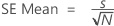
Standard error of the mean (SE Mean)
The standard error of the mean is calculated as the standard deviation divided by the square root of the sample size.
Formula
Notation
| Term | Description |
|---|---|
| s | standard deviation of the sample |
| N | number of nonmissing observations |
Standard deviation (StDev)
The sample standard deviation provides a measure of the spread of your data. It is equal to the square root of the sample variance.
Formula
 , then the standard deviation of the sample is:
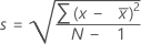
Notation
| Term | Description |
|---|---|
| x i | i th observation |
 | mean of the observations |
| N | number of nonmissing observations |
Variance
The variance measures how spread out the data are about their mean. The variance is equal to the standard deviation squared.
Formula
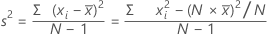
Notation
| Term | Description |
|---|---|
| xi | ith observation |
 | mean of the observations |
| N | number of nonmissing observations |
Coefficient of variation (CoefVar)
The coefficient of variation is a measure of relative variability calculated as a percentage.
Formula

Minitab calculates it as:

Notation
| Term | Description |
|---|---|
| s | standard deviation of the sample |
 | mean of the observations |
1st quartile (Q1)
25% of your sample observations are less than or equal to the value of the 1st quartile. Therefore, the 1st quartile is also referred to as the 25th percentile.
Formula

Notation
| Term | Description |
|---|---|
| y | truncated integer value of w |
| w |  |
| z | fraction component of w that was truncated |
| xj | jth observation in the list of sample data, ordered from smallest to largest |
Note
When w is an integer, y = w, z = 0, and Q1 = xy.
Median
The sample median is in the middle of the data: at least half the observations are less than or equal to it, and at least half are greater than or equal to it.
Suppose you have a column that contains N values. To calculate the median, first order your data values from smallest to largest. If N is odd, the sample median is the value in the middle. If N is even, the sample median is the average of the two middle values.
For example, when N = 5 and you have data x1, x2, x3, x4, and x5, the median = x3.
When N = 6 and you have ordered data x1, x2, x3, x4, x5,and x6:
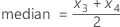
where x3 and x4 are the third and fourth observations.
3rd quartile (Q3)
75% of your sample observations are less than or equal to the value of the third quartile. Therefore, the third quartile is also referred to as the 75th percentile.
Formula

Notation
| Term | Description |
|---|---|
| y | truncated value of w |
| w |
 |
| z | fraction component of w that was truncated away |
| xj | jth observation in the list of sample data, ordered from smallest to largest |
Note
When w is an integer, y = w, z = 0, and Q3 = xy.
Interquartile range (IQR)
The interquartile range equals the third quartile minus the 1st quartile.
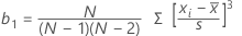
Mode
The mode is the data value that occurs most often in the dataset. If multiple modes exist, Minitab displays the smallest modes, up to a total of four. N for Mode is the number of times the mode (or modes) appears.
Trimmed mean (TrMean)
Minitab calculates the trimmed mean by removing the smallest 5% and the largest 5% of the values (rounded to the nearest integer), and then calculating the mean of the remaining values.
Sum
Formula

Notation
| Term | Description |
|---|---|
| xi | i th observation |
Minimum
The smallest value in your data set.
Maximum
The largest value in your data set.
Range
The range is calculated as the difference between the largest and smallest data value.
R = Maximum – Minimum
Sum of squares
Minitab squares each value in the column, then computes the sum of those squared values.
Formula

Notation
| Term | Description |
|---|---|
| xi | i th observation |
Skewness
Skewness is a measure of asymmetry. A negative value indicates skewness to the left, and a positive value indicates skewness to the right. A zero value does not necessarily indicate symmetry.
Formula
Notation
| Term | Description |
|---|---|
| xi | i th observation |
 | mean of the observations |
| N | number of nonmissing observations |
| s | standard deviation of the sample |
Kurtosis
Kurtosis is one measure of how different a distribution is from the normal distribution. A positive value usually indicates that the distribution has a sharper peak than the normal distribution. A negative value indicates that the distribution has a flatter peak than the normal distribution.
Formula

Notation
| Term | Description |
|---|---|
| xi | i th observation |
 | mean of the observations |
| N | number of nonmissing observations |
| s | standard deviation of the sample |
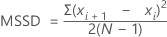
MSSD (mean of the squared successive differences)
Minitab calculates half the MSSD (mean of the squared successive differences) of a batch of numbers. The successive differences are squared and summed. Then Minitab divides by 2 and calculates the average.
Formula
Notation
| Term | Description |
|---|---|
| xi | i th observation |
 | mean of the observations |
N nonmissing (N)
The number of non-missing values in the sample.
N missing (N*)
The number of missing values in the sample. The number of missing values refers to cells that contain the missing value symbol *.
N total (total count)
The total number of observations in the column.
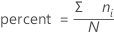
Percent
Minitab calculates what percentage of the whole that is accounted for by each group.
Formula
Notation
| Term | Description |
|---|---|
| ni | number of observations in the ith group |
| N | number of nonmissing observations |
Cumulative percent (CumPct)
Minitab calculates the cumulative percentage that is represented by each group.
Formula

Notation
| Term | Description |
|---|---|
| ni | number of observations in the ith group |
| N | number of nonmissing observations |