In This Topic
Step 1: Examine the relationships between variables on a matrix plot
Use the matrix plot to examine the relationships between two continuous variables. Also, look for outliers in the relationships. Outliers can heavily influence the results for the Pearson correlation coefficient.
Determine whether the relationships are linear, monotonic, or neither. The following are examples of the types of forms that the correlation coefficients describe. The Pearson correlation coefficient is appropriate for linear forms. Spearman's correlation coefficient is appropriate for monotonic forms.
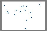
No relationship
The points fall randomly on the plot, which indicates that there is no linear relationship between the variables.
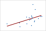
Moderate positive relationship
Some points are close to the line but other points are far from it, which indicates only a moderate linear relationship between the variables.
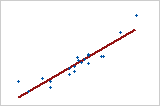
Large positive relationship
The points fall close to the line, which indicates that there is a strong linear relationship between the variables. The relationship is positive because as one variable increases, the other variable also increases.
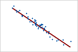
Large negative relationship
The points fall close to the line, which indicates that there is a strong negative relationship between the variables. The relationship is negative because, as one variable increases, the other variable decreases.
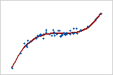
Monotonic
In a monotonic relationship, the variables tend to move in the same relative direction, but not necessarily at a constant rate. In a linear relationship, the variables move in the same direction at a constant rate. This plot shows both variables increasing concurrently, but not at the same rate. This relationship is monotonic, but not linear. The Pearson correlation coefficient for these data is 0.843, but the Spearman correlation is higher, 0.948.
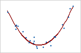
Curved quadratic
This example shows a curved relationship. Even though the relationship between the variables is strong, the correlation coefficient would be close to zero. The relationship is neither linear nor monotonic.
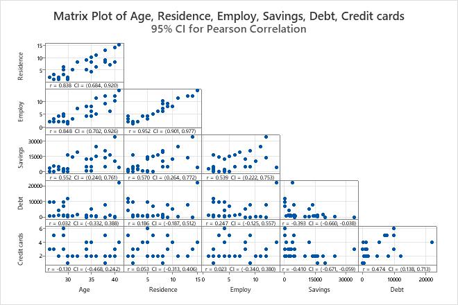
Key Result: Matrix Plot
- A strong positive linear relationship exists between Employ and Residence.
- A weak negative linear relationship exists between Credit cards and Savings.
- Debt seems to have an outlier which should be investigated.
Step 2: Examine the correlation coefficients between variables
Use the Pearson correlation coefficient to examine the strength and direction of the linear relationship between two continuous variables.
- Strength
-
The correlation coefficient can range in value from −1 to +1. The larger the absolute value of the coefficient, the stronger the relationship between the variables.
For the Pearson correlation, an absolute value of 1 indicates a perfect linear relationship. A correlation close to 0 indicates no linear relationship between the variables. - Direction
-
The sign of the coefficient indicates the direction of the relationship. If both variables tend to increase or decrease together, the coefficient is positive, and the line that represents the correlation slopes upward. If one variable tends to increase as the other decreases, the coefficient is negative, and the line that represents the correlation slopes downward.
- It is never appropriate to conclude that changes in one variable cause changes in another based on correlation alone. Only properly controlled experiments enable you to determine whether a relationship is causal.
- The Pearson correlation coefficient is very sensitive to extreme data values. A single value that is very different from the other values in a data set can greatly change the value of the coefficient. You should try to identify the cause of any extreme value. Correct any data entry or measurement errors. Consider removing data values that are associated with abnormal, one-time events (special causes). Then, repeat the analysis.
- A low Pearson correlation coefficient does not mean that no relationship exists between the variables. The variables may have a nonlinear relationship.
Method
| Correlation type | Pearson |
|---|---|
| Number of rows used | 30 |
Correlations
| Age | Residence | Employ | Savings | Debt | |
|---|---|---|---|---|---|
| Residence | 0.838 | ||||
| Employ | 0.848 | 0.952 | |||
| Savings | 0.552 | 0.570 | 0.539 | ||
| Debt | 0.032 | 0.186 | 0.247 | -0.393 | |
| Credit cards | -0.130 | 0.053 | 0.023 | -0.410 | 0.474 |
Key Result: Pearson correlation
- Residence and Age, 0.838
- Employ and Age, 0.848
- Employ and Residence, 0.952
- Debt and Savings , −0.393
- Credit cards and Age, −0.130
- Credit cards and Savings, −0.410