Step 1: Examine the shape of your bootstrap distribution
Use the histogram to examine the shape of your bootstrap distribution. The bootstrap distribution is the distribution of the chosen statistic from each resample. The bootstrap distribution should appear to be normal. If the bootstrap distribution is non-normal, you cannot trust the bootstrap results.
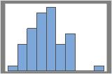
50 resamples
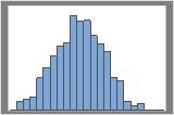
1000 resamples
The distribution is usually easier to determine with more resamples. For example, in these data, the distribution is ambiguous for 50 resamples. With 1000 resamples, the shape looks approximately normal.
In this histogram, the bootstrap distribution appears to be normal.
Step 2: Determine whether the test results are statistically significant
To determine whether the difference between population means is statistically significant, compare the p-value to the significance level. Usually, a significance level (denoted as α or alpha) of 0.05 works well. A significance level of 0.05 indicates a 5% risk of concluding that a difference exists when there is no actual difference.
P-value ≤ α: The difference between the means is statistically significant (Reject H0)
If the p-value is less than or equal to the significance level, the decision is to reject the null hypothesis. You can conclude that the difference between the population means is statistically significant. To calculate a confidence interval and determine whether the difference is practically significant, use Bootstrapping
for 2-sample means. For more information, go to Statistical and practical significance.
P-value > α: The difference between the means is not statistically significant (Fail to reject H0)
If the p-value is greater than the significance level, the decision is to fail to reject the null hypothesis. You do not have enough evidence to conclude that the difference between the population means is statistically significant.
Method
μ₁: population mean of Rating when Hospital = A
µ₂: population mean of Rating when Hospital = B
Difference: μ₁ - µ₂
Observed Samples
Hospital
N
Mean
StDev
Variance
Minimum
Median
Maximum
A
20
80.30
8.18
66.96
62.00
79.00
98.00
B
20
59.30
12.43
154.54
35.00
58.50
89.00
Difference in Observed Means
Mean of A - Mean of B = 21.000
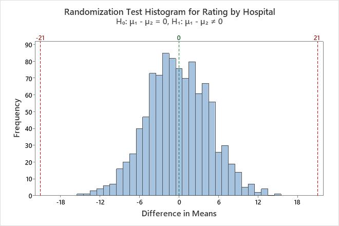
Randomization Test
Null hypothesis
H₀: μ₁ - µ₂ = 0
Alternative hypothesis
H₁: μ₁ - µ₂ ≠ 0
Number of Resamples
Average
StDev
P-Value
1000
-0.185
4.728
< 0.002
Key Results: P-Value
In these results, the null hypothesis states that the difference in the mean rating between two hospitals is 0. Because the p-value is less than 0.002, which is less than the significance level of 0.05, the decision is to reject the null hypothesis and conclude that the ratings of the hospitals are different.