Step 1: Examine the calculated values
Using the values of the two power function variables that you entered, Minitab calculates the difference, the sample size, or the power of the test.
- Difference
-
Minitab calculates the minimum difference for which you can achieve the specified level of power for each sample size. Larger sample sizes enable the test to detect smaller differences. You want to detect the smallest difference that has practical consequences for your application.
This value represents the difference between the actual population mean and the hypothesized mean.
- Sample size
-
Minitab calculates how large your sample must be for a test with your specified power to detect each specified difference. Because sample sizes are whole numbers, the actual power of the test might be slightly greater than the power value that you specify.
If you increase the sample size, the power of the test also increases. You want enough observations in your sample to achieve adequate power. But you don't want a sample size so large that you waste time and money on unnecessary sampling or detect unimportant differences to be statistically significant.
- Power
-
Minitab calculates the power of the test based on the specified difference and sample size. A power value of 0.9 is usually considered adequate. A value of 0.9 indicates that you have a 90% chance of detecting a difference between the population mean and the target when a difference actually exists. If a test has low power, you might fail to detect a difference and mistakenly conclude that none exists. Usually, when the sample size is smaller or the difference is smaller, the test has less power to detect a difference.
Results
| Difference | Sample Size | Target Power | Actual Power |
|---|---|---|---|
| 1.5 | 32 | 0.9 | 0.903816 |
Key Results: Difference, Sample Size, Power
These results show that if the difference is 1.5 and the power is 0.9, then you should collect a sample size of 32. Because the target power value of 0.9 results in a sample size that is not an integer, Minitab also displays the power (Actual Power) for the rounded sample size.
Step 2: Examine the power curve
Use the power curve to assess the appropriate sample size or power for your test.
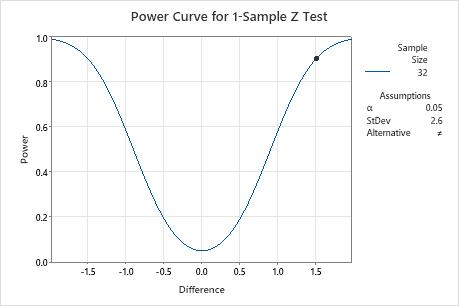
The power curve represents every combination of power and difference for each sample size when the significance level and the standard deviation are held constant. Each symbol on the power curve represents a calculated value based on the values that you enter. For example, if you enter a sample size and a power value, Minitab calculates the corresponding difference and displays the calculated value on the graph.
Examine the values on the curve to determine the difference between the mean and the target that can be detected at a certain power value and sample size. A power value of 0.9 is usually considered adequate. However, some practitioners consider a power value of 0.8 to be adequate. If a hypothesis test has low power, you might fail to detect a difference that is practically significant. If you increase the sample size, the power of the test also increases. You want enough observations in your sample to achieve adequate power. But you don't want a sample size so large that you waste time and money on unnecessary sampling or detect unimportant differences to be statistically significant. If you decrease the size of the difference that you want to detect, the power also decreases.
In this graph, the power curve for a sample size of 32 shows that the test has a power of 0.9 for a difference of 1.5. As the difference approaches 0, the power of the test decreases and approaches α (also called the significance level), which is 0.05 for this analysis.