In This Topic
Link function
Minitab provides three link functions: logit (the default), normit, and gompit. The link functions allow you to fit a broad class of ordinal response models. The logit is the inverse of the standard cumulative logistic distribution function. The normit function, also known as probit, is the inverse of the standard cumulative normal distribution function. The gompit function, also known as complementary log-log, is the inverse of the Gompertz distribution function.
Formula
g(χ k ) = θk +x'β, k = 1, ..., K-1
The link function is the inverse of a distribution function. The link functions and their corresponding distributions are summarized below:
| Name | Link Function | Distribution |
|---|---|---|
| logit | g(χ) = loge(χ/ (1 – χ)) | logistic |
| normit (probit) |
g(χ) = Φ–1(χ) |
normal |
| gompit (complementary log-log) | g(χ) =loge (–loge(1 – χ)) | Gompertz |
Notation
| Term | Description |
|---|---|
| K | number of distinct categories of the response |
| χk | cumulative probability up to and including category k, (π 1+ ...+ πk ) |
| g(χ k ) | vector of predictor variables |
| θk | constant associated with the kthdistinct response category |
| x | a vector of predictor variables |
| β | a vector of coefficients associated with the predictors |
Factor/covariate pattern
Describes a single set of factor/covariate values in a data set. Minitab calculates event probabilities, residuals, and other diagnostic measures for each factor/covariate pattern.
For example, if a data set includes the factors gender and race and the covariate age, the combination of these predictors may contain as many different covariate patterns as subjects. If a data set only includes the factors race and sex, each coded at two levels, there are only four possible factor/covariate patterns. If you enter your data as frequencies, or as successes, trials, or failures, each row contains one factor/covariate pattern.
Event probability
Event probabilities are the π k for k = 1, 2, ..., K.
Formula
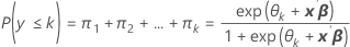
Notation
| Term | Description |
|---|---|
| k | equals 1, ..., K – 1 |
| θk | constant |
| β | vector of coefficients from the logit equation |
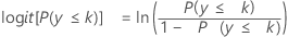
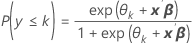
Cumulative event probability
The probability that the response falls into category k or below, for each possible k. The kth cumulative probability is:
Formula
P(y  k) = p1 + ... + p k , k = 1, ... , K
The cumulative probabilities reflect the order of the response. For a model with k response categories:
P(y  1) <P(y
  2)
2)  …
… P(y
P(y  K) = 1
Coefficient
Minitab uses the proportional odds model where a vector of predictors, x, has a parameter β describing the effect of x on the log odds of the response in category k or below. Minitab assumes an identical effect of x for all K – 1 categories, so only 1 coefficient is calculated for each predictor. The coefficient for the predictor indicates that for any fixed k, the estimated change in the logit of the response when predictor is at one level compared to the reference level.
Minitab estimates a constant for each K – 1 category. Use the parameter estimates to calculate estimated probabilities for each category using the model for the cumulative probabilities:
Formula
The estimated coefficients are calculated using an iterative reweighted least squares method, which is equivalent to maximum likelihood estimation.1,2
References
- D.W. Hosmer and S. Lemeshow (2000). Applied Logistic Regression. 2nd ed. John Wiley & Sons, Inc.
- P. McCullagh and J.A. Nelder (1992). Generalized Linear Model. Chapman & Hall.
Standard error of coefficients
Asymptotic standard error, which indicates the precision of the estimated coefficient. The smaller the standard error, the more precise the estimate.
See [1] and [2] for more information.
- A. Agresti (1990). Categorical Data Analysis. John Wiley & Sons, Inc.
- P. McCullagh and J.A. Nelder (1992). Generalized Linear Model. Chapman & Hall.
Z
Z is used to determine whether the predictor is significantly related to the response. Larger absolute values of Z indicate a significant relationship. The p-value indicates where Z falls on the normal distribution.
Formula
Z = βi / standard error
The formula for the constant is:
Z = θk / standard error
For small samples, the likelihood-ratio test may be a more reliable test of significance.
p-value (P)
Used in hypothesis tests to help you decide whether to reject or fail to reject a null hypothesis. The p-value is the probability of obtaining a test statistic that is at least as extreme as the actual calculated value, if the null hypothesis is true. A commonly used cut-off value for the p-value is 0.05. For example, if the calculated p-value of a test statistic is less than 0.05, you reject the null hypothesis.
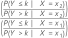
Odds ratio
Minitab uses a proportional odds model for ordinal logistic regression. Only one parameter and one odds ratio is calculated for each predictor. The odds ratio utilizes cumulative probabilities and their complements. For a predictor with 2 levels x 1 and x 2, the cumulative odds ratio is:
Formula
Confidence interval
Formula
The large sample confidence interval for βi is:
β i + Zα /2* (standard error)
To obtain the confidence interval of the odds ratio, exponentiate the lower and upper limits of the confidence interval. The interval provides the range in which the odds may fall for every unit change in the predictor.
Notation
| Term | Description |
|---|---|
| α | significance level |
Log-likelihood
Derived from the individual probability density functions, the expression is maximized to yield optimal values of β. The log-likelihood cannot be used alone as a measure of fit because it depends on sample size but can be used to compare two models.
For ordinal logistic regression, there are n independent multinomial vectors, each with k categories. These observations are denoted by y 1, ..., y n, where yi = (y i1, ..., yik ) and Σ j yij = mi is fixed for each i. From the ith observation yi , the contribution to the log likelihood is:
Formula
L(πi ; yi ) = Σ k yik log πik
The total log likelihood is a sum of contributions from each of the n observations:
L(π ; y) = Σ i L(πi ; yi )
Notation
| Term | Description |
|---|---|
| πik | probability of the ith observation for the kth category |
Variance-covariance matrix
A square matrix with the dimensions p + K – 1. The variance of each coefficient is in the diagonal cell and the covariance of each pair of coefficients is in the appropriate off-diagonal cell. The variance is the standard error of the coefficient squared.
The variance-covariance matrix is asymptotic and is obtained from the final iteration of the inverse of the information matrix.
Notation
| Term | Description |
|---|---|
| p | number of predictors |
| K | number of categories in the response |
Pearson
A summary statistic based on the Pearson residuals that indicates how well the model fits your data. Pearson isn't useful when the number of distinct values of the covariate is approximately equal to the number of observations, but is useful when you have repeated observations at the same covariate level. Higher χ2 test statistics and lower p-values values indicate that the model may not fit the data well.
The formula is:

where r = Pearson residual, m = number of trials in the jth factor/covariate pattern, and π0 = hypothesized value for the proportion.
Deviance
A summary statistic based on the Deviance residuals that indicates how well the model fits your data. Deviance isn't useful when the number of distinct values of the covariate is approximately equal to the number of observations, but is useful when you have repeated observations at the same covariate level. Higher values of D and lower p-values values indicate that the model may not fit the data well. The degrees of freedom for the test is (k - 1)*J − (p) where k is the number categories in the response, J is the number of distinct factor/covariate patterns and p is the number of coefficients.
The formula is:
D =2 Σ yik log p ik− 2 Σ yik log π ik
where πik = probability of the ith observation for the kth category.
Measures of association
Concordant and discordant pairs indicate how well your model predicts data. The more concordant pairs you have, the better your model's predictive ability.
The table of concordant, discordant, and tied pairs is calculated by forming all possible pairs of observations with different response values. Suppose the response values are 1, 2, and 3. Minitab pairs every observation with response value 1 with every observation with response values of 2 and 3 and then pairs every observation with the response value 2 with every observation with response values 1 and 3. The total number of pairs equals the number of observations with response of 1 multiplied by the number of observations with the response of 2 plus the number of observations with response of 1 multiplied by the number of observations with the response of 3 plus the number of observations with response of 2 multiplied by the number of observations with the response of 3.
To determine whether the pairs are concordant or discordant, Minitab calculates the cumulative predicted probabilities of each observation and compares these values for each pair of observations.
- Concordant
- For pairs that include the lowest response value (in the example above, that is 1), a pair is concordant if the cumulative probability up to the lowest response value is greater for the observation with the lowest response value than for the observation with the higher response value. For pairs with the highest response values (in the example above, pairs with 2 and 3), a pair is concordant if the cumulative probability up to 2 is greater for the observation with the response value 2 than the observation with the response value 3.
- Discordant
- For pairs that include the lowest response value (in the example above, that is 1), a pair is discordant if the cumulative probability up to the lowest response value is greater for the observation with the higher response value than for the observation with the lower response value. For pairs with the highest response values (in the example above, pairs with 2 and 3), a pair is discordant if the cumulative probability up to 2 is greater for the observation with the response value 3 than the observation with the response value 2.
- Ties
- A pair is tied if the observations have equal cumulative probabilities.
Formula
From the table of concordant, discordant, and tied pairs, Minitab calculates the following summary measures:


Notation
| Term | Description |
|---|---|
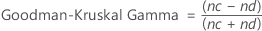
| nc | number of concordant pairs |
| nd | number of discordant pairs |
| nt | number of tied pairs |
| N | total number of observations |