In This Topic
DF
The degrees of freedom (DF) for each SS (sums of squares). In general, DF measures how much information is available to calculate each SS.
Seq SS
The sequential sum of squares for each term in the model (factor or interaction) measures the amount of variation in the response that is explained by adding each term to the model sequentially in the order listed under source. Thus, the sequential sums of squares for terms are specific to the order of the terms specified in the model.
SS Total = SS Part + SS Operator + SS Other Factors + SS Operator * Part + SS Other Interactions + SS Repeatability
Adj SS
The adjusted sum of squares are measures of variation for different components in the model. The order of the terms (factors or interactions) in the model does not affect the calculation of the adjusted sum of squares. In the ANOVA table, Minitab separates the sum of squares into different components that describe variation due to different sources.
Adj MS
The adjusted mean squares measure how much variation a term or a model explains, assuming that all other terms are in the model, regardless of the order they were entered. Unlike adjusted sums of squares, adjusted mean squares consider the degrees of freedom.
Adj MS = Adj SS/DF for each source of variability
Minitab uses the adjusted mean square to calculate the p-value for a term.
F
The statistic that is used to determine whether the factor effects, such as Operator and Part, and the interaction effects, such as Operator*Part, are statistically significantly.
The larger the F statistic, the more likely it is that the factor contributes significantly to the variability in the response or measurement variable.
P
The p-value is the probability of obtaining a test statistic (such as the F-statistic) that is at least as extreme as the value that is calculated from the sample, if the null hypothesis is true.
Interpretation
Use the p-value in the ANOVA table to determine whether the average measurements are significantly different. Minitab displays an ANOVA table only if you select the ANOVA option for Method of Analysis.
A low p-value indicates that the assumption of all parts, operators, or interactions sharing the same mean is probably not true.
- P-value ≤ α: At least one mean is statistically different
- If the p-value is less than or equal to the significance level, you reject the null hypothesis and conclude that at least one of the means is significantly different from the others. For example, at least one operator measures differently.
- P-value > α: The means are not significantly different
- If the p-value is greater than the significance level, you fail to reject the null hypothesis because you do not have enough evidence to conclude that the population means are different. For example, you can not conclude that the operators measure differently.
VarComp
VarComp is the estimated variance components for each source in an ANOVA table.
Interpretation
Use the variance components to assess the variation for each source of measurement error.
In an acceptable measurement system, the largest component of variation is Part-to-Part variation. If repeatability and reproducibility contribute large amounts of variation, you need to investigate the source of the problem and take corrective action.
%Contribution (of VarComp)
%Contribution is the percentage of overall variation from each variance component. It is calculated as the variance component for each source divided by the total variation, then multiplied by 100 to express as a percentage.
Interpretation
Use the %Contribution to assess the variation for each source of measurement error.
In an acceptable measurement system, the largest component of variation is Part-to-Part variation. If repeatability and reproducibility contribute large amounts of variation, you need to investigate the source of the problem and take corrective action.
StdDev (SD)
StdDev (SD) is the standard deviation for each source of variation. The standard deviation is equal to the square root of the variance component for that source.
The standard deviation is a convenient measure of variation because it has the same units as the part measurements and tolerance.
Study Var (6 * SD)
The study variation is calculated as the standard deviation for each source of variation multiplied by 6 or the multiplier that you specify in Study variation.
Usually, process variation is defined as 6s, where s is the standard deviation as an estimate of the population standard deviation (denoted by σ or sigma). When data are normally distributed, approximately 99.73% of the data fall within 6 standard deviations of the mean. To define a different percentage of data, use another multiplier of standard deviation. For example, if you want to know where 99% of the data fall, you would use a multiplier of 5.15, instead of the default multiplier of 6.
%Study Var (%SV)
The %study variation is calculated as the study variation for each source of variation, divided by the total variation and multiplied by 100.
%Study Var is the square root of the calculated variance component (VarComp) for that source. Thus, the %Contribution of VarComp values sum to 100, but the %Study Var values do not.
Interpretation
Use %Study Var to compare the measurement system variation to the total variation. If you use the measurement system to evaluate process improvements, such as reducing part-to-part variation, %Study Var is a better estimate of measurement precision. If you want to evaluate the capability of the measurement system to evaluate parts compared to specification, %Tolerance is the appropriate metric.
%Tolerance (SV/Toler)
%Tolerance is calculated as the study variation for each source, divided by the process tolerance and multiplied by 100.
If you enter the tolerance, Minitab calculates %Tolerance, which compares measurement system variation to the specifications.
Interpretation
Use %Tolerance to evaluate parts relative to specifications. If you use the measurement system for process improvement, such as reducing part-to-part variation, %StudyVar is the appropriate metric.
%Process (SV/Proc)
If you enter a historical standard deviation but use the parts in the study to estimate the process variation, then Minitab calculates %Process. %Process compares measurement system variation to the historical process variation. %Process is calculated as the study variation for each source, divided by the historical process variation and multiplied by 100. By default, the process variation is equal to 6 times the historical standard deviation.
If you use a historical standard deviation to estimate process variation, then Minitab does not show %Process because %Process is identical to %Study Var.
Number of distinct categories
The number of distinct categories is a metric that is used in gage R&R studies to identify a measurement system's ability to detect a difference in the measured characteristic. The number of distinct categories represents the number of non-overlapping confidence intervals that span the range of product variation, as defined by the samples that you chose. The number of distinct categories also represents the number of groups within your process data that your measurement system can discern.
Interpretation
The Measurement Systems Analysis Manual1 published by the Automobile Industry Action Group (AIAG) states that 5 or more categories indicates an acceptable measurement system. If the number of distinct categories is less than 5, the measurement system might not have enough resolution.
Usually, when the number of distinct categories is less than 2, the measurement system is of no value for controlling the process, because it cannot distinguish between parts. When the number of distinct categories is 2, you can split the parts into only two groups, such as high and low. When the number of distinct categories is 3, you can split the parts into 3 groups, such as low, middle, and high.
For more information, go to Using the number of distinct categories.
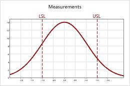
Probabilities of misclassification
When you specify at least one specification limit, Minitab can calculate the probabilities of misclassifying product. Because of the gage variation, the measured value of the part does not always equal the true value of the part. The discrepancy between the measured value and the actual value creates the potential for misclassifying the part.
- Joint probability
- Use the joint probability when you don't have prior knowledge about the acceptability of the parts. For example, you are sampling from the line and don't know whether each particular part is good or bad. There are two misclassifications that you can make:
- The probability that the part is bad, and you accept it.
- The probability that the part is good, and you reject it.
- Conditional probability
- Use the conditional probability when you do have prior knowledge about the acceptability of the parts. For example, you are sampling from a pile of rework or from a pile of product that will soon be shipped as good. There are two misclassifications that you can make:
- The probability that you accept a part that was sampled from a pile of bad product that needs to be reworked (also called false accept).
- The probability that you reject a part that was sampled from a pile of good product that is about to be shipped (also called false reject).
Interpretation
Joint Probability
| Description | Probability |
|---|---|
| A randomly selected part is bad but accepted | 0.037 |
| A randomly selected part is good but rejected | 0.055 |
Conditional Probability
| Description | Probability |
|---|---|
| A part from a group of bad products is accepted | 0.151 |
| A part from a group of good products is rejected | 0.073 |
The joint probability that a part is bad and you accept it is 0.037. The joint probability that a part is good and you reject it is 0.055.
The conditional probability of a false accept, that you accept a part during reinspection when it is really out-of-specification, is 0.151. The conditional probability of a false reject, that you reject a part during reinspection when it is really in-specification, is 0.073.
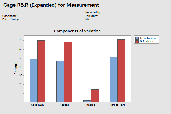
Components of variation graph
The components of variation chart is a graphical summary of the results of a gage R&R study.
- Total Gage R&R: The variability from the measurement system that includes multiple operators using the same gage.
- Repeatability: The variability in measurements when the same operator measures the same part multiple times.
- Reproducibility: The variability in measurements when different operators measure the same part.
- Part-to-Part: The variability in measurements due to different parts.
Interpretation
- %Contribution
- %Contribution is the percentage of overall variation from each variance component. It is calculated as the variance component for each source divided by the total variation, then multiplied by 100.
- %Study Variation
- %Study Variation is the percentage of study variation from each source. It is calculated as the study variation for each source divided by the total study variation, then multiplied by 100.
- %Tolerance
- %Tolerance compares measurement system variation to specifications. It is calculated as the study variation for each source divided by the process tolerance, then multiplied by 100.
- %Process
- %Process compares measurement system variation to the total variation. It is calculated as the study variation for each source divided by the historical process variation, then multiplied by 100.
In an acceptable measurement system, the largest component of variation is part-to-part variation.
Xbar chart
The Xbar chart compares the part-to-part variation to the repeatability component.
- Plotted points
- The average measurement of each part, plotted by each operator.
- Center line (Xbar)
- The overall average for all part measurements by all operators.
- Control limits (LCL and UCL)
- The control limits are based on the repeatability estimate and the number of measurements in each average.
Interpretation
The parts that are chosen for a Gage R&R study should represent the entire range of possible parts. Thus, this graph should indicate more variation between part averages than what is expected from repeatability variation alone.
Ideally, the graph has narrow control limits with many out-of-control points that indicate a measurement system with low variation.
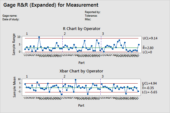
R chart
The R chart is a control chart of ranges that displays operator consistency.
- Plotted points
- For each operator, the difference between the largest and smallest measurements of each part. The R chart plots the points by operator so you can see how consistent each operator is.
- Center line (Rbar)
- The grand average for the process (that is, average of all the sample ranges).
- Control limits (LCL and UCL)
- The amount of variation that you can expect for the sample ranges. To calculate the control limits, Minitab uses the variation within samples.
Note
If each operator measures each part 9 times or more, Minitab displays an S chart instead of an R chart.
Interpretation
A small average range indicates that the measurement system has low variation. A point that is higher than the upper control limit (UCL) indicates that the operator does not measure parts consistently. The calculation of the UCL includes the number of measurements per part by each operator, and part-to-part variation. If the operators measure parts consistently, then the range between the highest and lowest measurements is small, relative to the study variation, and the points should be in control.
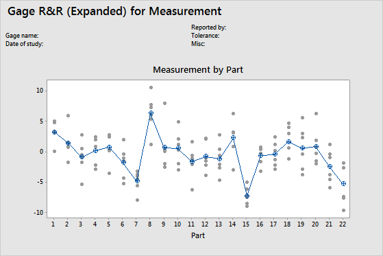
By Single Factor (Part) graph
The By Part graph displays all measurements arranged by part so that you can see the differences between parts. Gage R&R studies usually arrange measurements by part and by operator, but with an expanded gage R&R study, you can graph other factors.
In the graph, dots represent the measurements, and circle-cross symbols represent the means. The connect line connects the average measurements for each factor level.
Note
If there are more than 9 observations per level, Minitab displays a boxplot instead of an individual value plot.
Interpretation
Multiple measurements for each individual part that vary as minimally as possible (the dots for one part are close together) indicate that the measurement system has low variation. Also, the average measurements of the parts should vary enough to show that the parts are different and represent the entire range of the process.
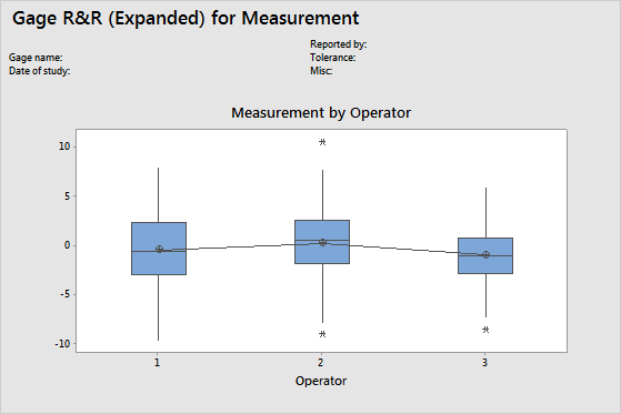
By Single Factor (Operator) graph
The By Operator graph displays all the measurements, arranged by operator so that you can see the differences between operators. Gage R&R studies usually arrange measurements by part and by operator, but with an expanded gage R&R study, you can graph other factors.
Note
If there are less than 10 observations per operator, Minitab displays an individual value plot instead of a boxplot.
Interpretation
A straight horizontal line across operators indicates that the mean measurements for each operator are similar. Ideally, the measurements for each operator vary an equal amount.
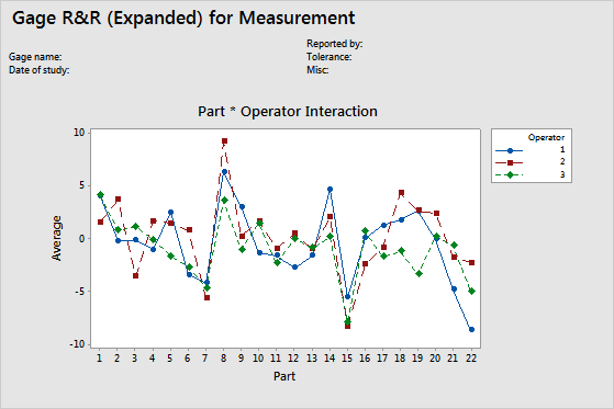
Interaction (Operator*Part) graph
The Operator* Part Interaction graph displays the average measurements by each operator for each part. Gage R&R studies usually include operator by part interactions, but with an expanded gage R&R study, you can graph other interactions.
Interaction plots display the interaction between two factors. An interaction occurs when the effect of one factor is dependent on a second factor. This plot is the graphical analog of the F-test for an interaction term in the ANOVA table.
Each line connects the averages for a single operator (or for a term that you specify).
Interpretation
Lines that are coincident indicate that the operators measure similarly. Lines that are not parallel or that cross indicate that an operator's ability to measure a part consistently depends on which part is being measured. A line that is consistently higher or lower than the others indicates that an operator adds bias to the measurement by consistently measuring high or low.