In This Topic
Weighted regression
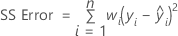
Weighted least squares regression is a method for dealing with observations that have nonconstant variances. If the variances are not constant, observations with:
- large variances should be given relatively small weights
- small variances should be given relatively large weights
The usual choice of weights is the inverse of pure error variance in the response.

Notation
| Term | Description |
|---|---|
| X | design matrix |
| X' | transpose of the design matrix |
| W | an n x n matrix with the weights on the diagonal |
| Y | vector of response values |
| n | number of observations |
| wi | weight for the ith observation |
| yi | response value for the ith observation |
 | fitted value for the ith observation |
Box-Cox transformation
Box-Cox transformation selects lambda values, as shown below, which minimize the residual sum of squares. The resulting transformation is Y λ when λ ≠ 0 and ln(Y) when λ = 0. When λ < 0, Minitab also multiplies the transformed response by −1 to maintain the order from the untransformed response.
Minitab searches for an optimal value between −2 and 2. Values that fall outside of this interval might not result in a better fit.
Here are some common transformations where Y′ is the transform of the data Y:
| Lambda (λ) value | Transformation |
|---|---|
| λ = 2 | Y′ = Y 2 |
| λ = 0.5 | Y′ = |
| λ = 0 | Y′ = ln(Y ) |
| λ = −0.5 | |
| λ = −1 | Y′ = −1 / Y |
Regression equation
For a model with multiple predictors, the equation is:
y = β0 + β1x1 + … + βkxk + ε
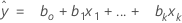
The fitted equation is:
In simple linear regression, which includes only one predictor, the model is:
y=ß0+ ß1x1+ε
Using regression estimates b0 for ß0, and b1 for ß1, the fitted equation is:

Notation
| Term | Description |
|---|---|
| y | response |
| xk | kth term. Each term can be a single predictor, a polynomial term, or an interaction term. |
| ßk | kth population regression coefficient |
| ε | error term that follows a normal distribution with a mean of 0 |
| bk | estimate of kth population regression coefficient |
 | fitted response |
Design matrix
The design matrix contains the predictors in a matrix (X) with n rows, where n is the number of observations. There is a column for each coefficient in the model.
Categorical predictors are coded using either 1, 0 or -1, 0, 1 coding. X does not include a column for the reference level of the factor.
To calculate the columns for an interaction term, multiply all of the corresponding values for the predictors in the interaction. For example, suppose the first observation has a value of 4 for predictor A and a value of 2 for predictor B. In the design matrix, the interaction between A and B is represented as 8 (4 x 2).
x'x inverse
How Minitab removes highly correlated predictors from the regression equation in Fit Regression Model
Let rij be the element in the current swept matrix associated with Xi and Xj.
Variables are entered or removed one at a time. Xk is eligible for entry if it is an independent variable not currently in the model with rkk ≥ 1 (tolerance with a default of 0.0001) and also for each variable Xj that is currently in the model,
- Minitab performs the SWEEP method on the correlation matrix, R, treating X1 … Xp as if they are random variables.
- For any continuous predictor, Minitab compares the element rkk with the tolerance; rkk ≥ tolerance, where k = 1 to p.
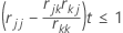
- For each variable Xj currently in the model, Minitab checks that (rjj – rjk * (rkj / rkk)) * tolerance ≤ 1.
Note
Where rkk, rjk, rjj are the corresponding diagonal and off diagonal elements for Xj and Xk variables after k step SWEEP operations.
- Otherwise, the predictor fails the test and is removed from the model.
Note
The default tolerance value is 8.8e–12.
Note
You can use the TOLERANCE subcommand with the REGRESS session command to force Minitab to keep a predictor in the model that is highly correlated with a different predictor. However, lowering the tolerance can be dangerous, possibly producing numerically inaccurate results.