In This Topic
Exponential family and link functions
The extension of the classical linear models to generalized linear models has two parts: a distribution from the exponential family and a link function.
The exponential family
The first part extends the linear model to response variables that are members of a large family of distributions called the exponential family. Members of the exponential family of distributions have probability distribution functions for an observed response in this general form:

where a(∙), b(∙), and c(∙) depend on the distribution of the response variable. The parameter θ is a location parameter that is often called the canonical parameter, and ϕ is called the dispersion parameter. The function a(ϕ) is usually of the form a(ϕ)= ϕ/ ω, where ω is a known constant or weight that may vary from one observation to another. (In Minitab, when weights are given the function a(ϕ), is adjusted accordingly.)
Members of the exponential family can be discrete distributions or continuous distributions. Examples of continuous distributions that are members of the exponential family are the normal and the gamma distributions. Examples of discrete distributions that are members of the exponential family are the binomial and the Poisson distributions. The following table gives the characteristics of some of these distributions.
| Distribution | ϕ | b(θ) | a(φ) | c(y, ϕ) |
| Normal | σ2 | θ2/2 | φω | 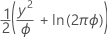 |
| Binomial | 1 |  |
φ/ω | -ln(y!) |
| Poisson | 1 | exp(θ) | φ/ω |  |
The link function
The second part is the link function. The link function relates the mean of the response in the ith observation to a linear predictor in this form:

The classical linear model is a special case of this general formulation where the link function is the identity function.
The choice of the link function in the second part depends upon the specific distribution of the exponential family of the first part. In particular, each distribution in the exponential family has a special link function called the canonical link function. This link function satisfies the equation g (μi) = Xi'β= θ, where θ is the canonical parameter. The canonical link function results in some desirable statistical properties of the model. Goodness-of-fit statistics can be used to compare fits using different link functions. Certain link functions may be used for historical reasons or because they have a special meaning in a discipline. For example, an advantage of the logit link function is that it provides an estimate of the odds ratios. Another example is that the normit link function assumes that there is an underlying variable that follows a normal distribution that is classified into binary categories.
Minitab provides three link functions for each class of models. The different link functions make it possible to find models that adequately fit a wider variety of data.
For binomial models, the link functions are logit, normit (also called probit), and gompit (also called complementary log-log). These are the inverse of the standard cumulative logistic distribution function (logit), the inverse of the standard cumulative normal distribution function (normit), and the inverse of the Gompertz distribution function (gompit). The logit is the canonical link function for binomial models, thus the logit is the default link function.
For Poisson models, the link functions are the natural log, the square root, and the identity. The natural log is the canonical link function for Poisson models, thus the natural log is the default link function.
The link functions are summarized below:
| Model | Name | Link Function, g(μi) |
| Binomial | logit |  |
| Binomial | normit (probit) |  |
| Binomial | gompit (complementary log-log) |  |
| Poisson | natural log |  |
| Poisson | square root |  |
| Poisson | identity |  |
Notation
| Term | Description |
|---|---|
| μi | the mean response of the ith row |
| g(μi) | the link function |
| X | the vector of predictor variables |
| β | the vector of coefficients associated with the predictors |
 | the inverse cumulative distribution function of the normal distribution |
Coefficients
[1] P. McCullagh and J. A. Nelder (1989). Generalized Linear Models, 2nd Ed., Chapman & Hall/CRC, London.
Standard error of coefficients

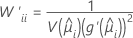
W is a diagonal matrix where the diagonal elements are given by the following formula:
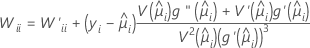
where

This variance-covariance matrix is based on the observed Hessian matrix as opposed to the Fisher's information matrix. Minitab uses the observed Hessian matrix because the model that results is more robust against any conditional mean misspecification.
If the canonical link is used then the observed Hessian matrix and the Fisher's information matrix are identical.
Notation
| Term | Description |
|---|---|
| yi | the response value for the ith row |
 | the estimated mean response for the ith row |
| V(·) | the variance function given in the table below |
| g(·) | the link function |
| V '(·) | the first derivative of the variance function |
| g'(·) | the first derivative of the link function |
| g''(·) | the second derivative of the link function |
The variance function depends on the model:
| Model | Variance function |
| Binomial |  |
| Poisson |  |
See [1] and [2] for more information.
[1] A. Agresti (1990). Categorical Data Analysis. John Wiley & Sons, Inc.
[2] P. McCullagh and J.A. Nelder (1992). Generalized Linear Model. Chapman & Hall.
Odds ratios for binary logistic regression
The odds ratio is provided only if you select the logit link function for a model with a binary response. In this case, the odds ratio is useful in interpreting the relationship between a predictor and a response.
The odds ratio (τ) can be any nonnegative number. The odds ratio = 1 serves as the baseline for comparison. If τ = 1, no association exists between the response and predictor. If τ < 1, the odds of the event are higher for the reference level of the factor (or for lower levels of a continuous predictor). If τ > 1, the odds of the event are less for the reference level of the factor (or for lower levels of a continuous predictor). Values farther from 1 represent stronger degrees of association.
Note
For the binary logistic regression model with one covariate or factor, the estimated odds of success are:
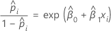
The exponential relationship provides an interpretation for β: The odds increase multiplicatively by eβ1 for every one-unit increase in x. The odds ratio is equivalent to exp(β1).
For example, if β is 0.75, the odds ratio is exp(0.75), which is 2.11. This indicates that there is a 111% increase in the odds of success for every one unit increase in x.
Notation
| Term | Description |
|---|---|
 | the estimated probability of a success for the ith row in the data |
 | the estimated intercept coefficient |
 | the estimated coefficient for predictor x |
 | the data point for the ith row |
Variance-covariance matrix
A d x d matrix, where d is the number of predictors plus one. The variance of each coefficient is in the diagonal cell and the covariance of each pair of coefficients is in the appropriate off-diagonal cell. The variance is the standard error of the coefficient squared.
The variance-covariance matrix is from the final iteration of the inverse of the information matrix. The variance-covariance matrix has the following form:

W is a diagonal matrix where the diagonal elements are given by the following formula:
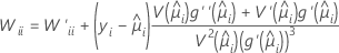
where
This variance-covariance matrix is based on the observed Hessian matrix as opposed to the Fisher's information matrix. Minitab uses the observed Hessian matrix because the model that results is more robust against any conditional mean misspecification.
If the canonical link is used then the observed Hessian matrix and the Fisher's information matrix are identical.
Notation
| Term | Description |
|---|---|
| yi | the response value for the ith row |
 | the estimated mean response for the ith row |
| V(·) | the variance function given in the table below |
| g(·) | the link function |
| V '(·) | the first derivative of the variance function |
| g'(·) | the first derivative of the link function |
| g''(·) | the second derivative of the link function |
The variance function depends on the model:
| Model | Variance function |
| Binomial |  |
| Poisson |  |
See [1] and [2] for more information.
[1] A. Agresti (1990). Categorical Data Analysis. John Wiley & Sons, Inc.
[2] P. McCullagh and J.A. Nelder (1992). Generalized Linear Model. Chapman & Hall.