Important predictors
Any classification tree is a collection of splits. Each split provides improvement to the tree. Each split also includes surrogate splits that also provide improvement to the tree. The importance of a variable is given by all of its improvements when the tree uses the variable to split a node or as a surrogate to split a node when another variable has a missing value.
The following formula gives the improvement at a single node:

The values of I(t), pLeft, and pRight depend on the criterion for splitting the nodes. For more information, go to Node splitting methods in CART® Classification.

Average –loglikelihood
Training data or no validation

where

Notation for training data or no validation
| Term | Description |
|---|---|
| N | sample size of the full data or the training data |
| wi | weight for the ith observation in the full or training data set |
| yi | indicator variable that is 1 for the event and 0 otherwise for the full or training data set |
 | predicted probability of the event for the ith row in the full or training data set |
K-fold cross-validation
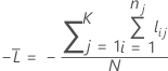
where

Notation for k-fold cross-validation
| Term | Description |
|---|---|
| N | sample size of the full or training data |
| nj | sample size of fold j |
| wij | weight for the ith observation in fold j |
| yij | indicator variable that is 1 for the event and 0 otherwise for the data in fold j |
 | predicted probability of the event from the model estimation that does not include the observations for the ith observation in fold j |
Test data set
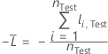
where

Notation for test data set
| Term | Description |
|---|---|
| nTest | sample size of the test set |
| wi, Test | weight for the ith observation in the test data set |
| yi, Test | indicator variable that is 1 for the event and 0 otherwise for the data in the test set |
 | predicted probability of the event for the ith row in the test set |
Area under ROC curve
Formula


For the area under the curve, Minitab uses an integration.

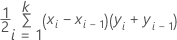
where k is the number of terminal nodes and (x0, y0) is the point (0, 0).
| x (false positive rate) | y (true positive rate) |
|---|---|
| 0.0923 | 0.3051 |
| 0.4154 | 0.7288 |
| 0.7538 | 0.9322 |
| 1 | 1 |


Notation
| Term | Description |
|---|---|
| TRP | true positive rate |
| FPR | false positive rate |
| TP | true positive, events that were correctly assessed |
| P | number of actual positive events |
| FP | true negative, nonevents that were correctly assessed |
| N | number of actual negative events |
| FNR | false negative rate |
| TNR | true negative rate |
95% CI for the area under the ROC curve
The following interval gives the upper and lower bounds for the confidence interval:

The computation of the standard error of the area under the ROC curve
( )
comes from Salford Predictive Modeler®. For general information
about estimation of the variance of the area under the ROC curve, see the
following references:
)
comes from Salford Predictive Modeler®. For general information
about estimation of the variance of the area under the ROC curve, see the
following references:
Engelmann, B. (2011). Measures of a ratings discriminative power: Applications and limitations. In B. Engelmann & R. Rauhmeier (Eds.), The Basel II Risk Parameters: Estimation, Validation, Stress Testing - With Applications to Loan Risk Management (2nd ed.) Heidelberg; New York: Springer. doi:10.1007/978-3-642-16114-8
Cortes, C. and Mohri, M. (2005). Confidence intervals for the area under the ROC curve. Advances in neural information processing systems, 305-312.
Feng, D., Cortese, G., & Baumgartner, R. (2017). A comparison of confidence/credible interval methods for the area under the ROC curve for continuous diagnostic tests with small sample size. Statistical Methods in Medical Research, 26(6), 2603-2621. doi:10.1177/0962280215602040
Notation
| Term | Description |
|---|---|
| A | area under the ROC curve |
 | 0.975 percentile of the standard normal distribution |
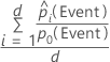
Lift
Formula
For the 10% of observations in the data with the highest probabilities of being assigned to the event class, use the following formula.
For the test lift with a test data set, use observations from the test data set. For the test lift with k-fold cross-validation, select the data to use and calculate the lift from the predicted probabilities for data that are not in the model estimation.
Notation
| Term | Description |
|---|---|
| d | number of cases in 10% of the data |
 | predicted probability of the event |
 | probability of the event in the training data or, if the analysis uses no validation, in the full data set |
Misclassification cost
The misclassification cost in the model summary table is the relative misclassification cost for the model relative to a trivial classifier that classifies all observations into the most frequent class.
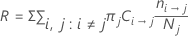
The relative misclassification cost has the following form:

Where R0 is the cost for the trivial classifier.
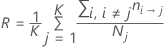
The formula for R simplifies when the prior probabilities are equal or are from the data.
Equal prior probabilities

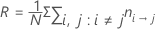
Prior probabilities from the data

With this definition, R has the following form:
Notation
| Term | Description |
|---|---|
| πj | prior probability of the jth class of the response variable |
 | cost of misclassifying class i as class j |
 | number of class i records misclassified as class j |
| Nj | number of cases in the jth class of the response variable |
| K | number of classes in the response variable |
| N | number of cases in the data |