A researcher tests the yields of six varieties of alfalfa on four randomly selected fields. The yield for each variety was recorded for each field.
The researcher wants to know whether the variety of alfalfa affects the mean yield. The researcher has 4 fields where they can collect data. However, the researcher wants to be able to model how the alfalfas will grow in fields that are not in the experiment. Thus, the researcher makes the field where the alfalfa grows a random factor. The researcher uses a mixed effects model to evaluate fixed and random effects together.
- Open the sample data Alfalfa.MWX.
- Choose .
- In Responses, enter Yield.
- In Random factors (required), enter Field.
- In Fixed factors, enter Variety.
- Click Graphs.
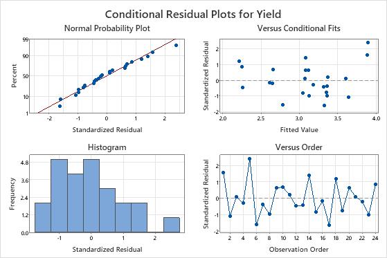
- In Residuals for plots, select Conditional standardized.
- In Residuals plots, select Four in one.
- Click OK in each dialog.
Interpret the results
In the Variance Components table, the p-value for Field is 0.124. The hypothesis test does not show evidence that the variance component is different from 0. The p-value for the variance component for error is 0.003. Because the p-value is less than the significance level of 0.05, the researcher can conclude that the variance component for error is not 0.
The p-value of approximately 0 for the fixed factor term, Variety, shows that at least one type of alfalfa effect on yield is significantly different from the other five types.
The coefficients for the main effects represent the difference between each level mean and the overall mean. For example, Variety 1 is associated with an alfalfa yield that is approximately 0.385 units greater than the overall mean. The p-value of approximately 0 for this coefficient indicates that the effect of Variety 1 on yield is significantly different from another level effect of the Variety term. To determine which level effects are statistically the same, and which level effects are statistically different, the researcher plans to do a multiple comparison analysis for the term.
The R2 value shows that the model explains about 92% of the variation in the yield. The R-sq (adj) value is also high, with a value of approximately 90.2%. The researcher uses this value to compare models that have different numbers of predictors.
Observation 1 and 5 are unusual observations because they have standardized residuals greater than 2. The researcher examines the data to make sure that the response values for those observations are correct.
The residuals on the normal probability plot approximate a straight line, and the points appear to be randomly scattered about 0 on the residuals versus fits plot.
Factor Information
| Factor | Type | Levels | Values |
|---|---|---|---|
| Field | Random | 4 | 1, 2, 3, 4 |
| Variety | Fixed | 6 | 1, 2, 3, 4, 5, 6 |
Variance Components
| Source | Var | % of Total | SE Var | Z-Value | P-Value |
|---|---|---|---|---|---|
| Field | 0.077919 | 72.93% | 0.067580 | 1.152996 | 0.124 |
| Error | 0.028924 | 27.07% | 0.010562 | 2.738613 | 0.003 |
| Total | 0.106843 |
Tests of Fixed Effects
| Term | DF Num | DF Den | F-Value | P-Value |
|---|---|---|---|---|
| Variety | 5.00 | 15.00 | 26.29 | 0.000 |
Model Summary
| S | R-sq | R-sq(adj) | AICc | BIC |
|---|---|---|---|---|
| 0.170071 | 92.33% | 90.20% | 12.54 | 13.52 |
Coefficients
| Term | Coef | SE Coef | DF | T-Value | P-Value |
|---|---|---|---|---|---|
| Constant | 3.094583 | 0.143822 | 3.00 | 21.516692 | 0.000 |
| Variety | |||||
| 1 | 0.385417 | 0.077626 | 15.00 | 4.965016 | 0.000 |
| 2 | 0.145417 | 0.077626 | 15.00 | 1.873287 | 0.081 |
| 3 | 0.107917 | 0.077626 | 15.00 | 1.390205 | 0.185 |
| 4 | -0.319583 | 0.077626 | 15.00 | -4.116938 | 0.001 |
| 5 | 0.395417 | 0.077626 | 15.00 | 5.093838 | 0.000 |
Marginal Fits and Diagnostics for Unusual Observations
| Obs | Yield | Fit | Resid | Std Resid | |
|---|---|---|---|---|---|
| 1 | 4.100000 | 3.480000 | 0.620000 | 2.190221 | R |
| 5 | 4.220000 | 3.490000 | 0.730000 | 2.578808 | R |
Conditional Fits and Diagnostics for Unusual Observations
| Obs | Yield | Fit | Resid | Std Resid | |
|---|---|---|---|---|---|
| 5 | 4.220000 | 3.895339 | 0.324661 | 2.400733 | R |