Fit
Fitted values are also called fits or  . The fitted values are point estimates of the mean response for given values of the predictors. The values of the predictors are also called x-values.
Interpretation
Fitted values are calculated by entering the specific x-values for each observation in the data set into the model equation.
For example, if the equation is y = 5 + 10x, the fitted value for the x-value, 2, is 25 (25 = 5 + 10(2)).
Observations with fitted values that are very different from the observed value may be unusual. Observations with unusual predictor values may be influential. If Minitab determines that your data include unusual or influential values, your output includes the table of Fits and Diagnostics for Unusual Observations, which identifies these observations. The unusual observations that Minitab labels do not follow the proposed regression equation well. However, it is expected that you will have some unusual observations. For example, based on the criteria for large standardized residuals, you would expect roughly 5% of your observations to be flagged as having a large standardized residual. For more information on unusual values, go to Unusual observations.
SE Fit
The standard error of the fit (SE fit) estimates the variation in the estimated mean response for the specified variable settings. The calculation of the confidence interval for the mean response uses the standard error of the fit. Standard errors are always non-negative.
Interpretation
Use the standard error of the fit to measure the precision of the estimate of the mean response. The smaller the standard error, the more precise the predicted mean response. For example, an analyst develops a model to predict delivery time. For one set of variable settings, the model predicts a mean delivery time of 3.80 days. The standard error of the fit for these settings is 0.08 days. For a second set of variable settings, the model produces the same mean delivery time with a standard error of the fit of 0.02 days. The analyst can be more confident that the mean delivery time for the second set of variable settings is close to 3.80 days.
With the fitted value, you can use the standard error of the fit to create a confidence interval for the mean response. For example, depending on the number of degrees of freedom, a 95% confidence interval extends approximately two standard errors above and below the predicted mean. For the delivery times, the 95% confidence interval for the predicted mean of 3.80 days when the standard error is 0.08 is (3.64, 3.96) days. You can be 95% confident that the population mean is within this range. When the standard error is 0.02, the 95% confidence interval is (3.76, 3.84) days. The confidence interval for the second set of variable settings is narrower because the standard error is smaller.
Resid
A residual (ei) is the difference between an observed value (y) and the corresponding fitted value, ( ), which is the value predicted by the model.
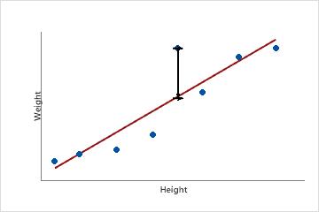
This scatterplot displays the weight versus the height for a sample of adult males. The fitted regression line represents the relationship between height and weight. If the height equals 6 feet, the fitted value for weight is 190 pounds. If the actual weight is 200 pounds, the residual is 10.
Interpretation
Plot the residuals to determine whether your model is adequate and meets the assumptions of regression. Examining the residuals can provide useful information about how well the model fits the data. In general, the residuals should be randomly distributed with no obvious patterns and no unusual values. If Minitab determines that your data include unusual observations, it identifies those observations in the Fits and Diagnostics for Unusual Observations table in the output. The observations that Minitab labels as unusual do not follow the proposed regression equation well. However, it is expected that you will have some unusual observations. For example, based on the criteria for large residuals, you would expect roughly 5% of your observations to be flagged as having a large residual. For more information on unusual values, go to Unusual observations.
Std Resid
The standardized residual equals the value of a residual (ei) divided by an estimate of its standard deviation.
Interpretation
Use the standardized residuals to help you detect outliers. Standardized residuals greater than 2 and less than −2 are usually considered large. The Fits and Diagnostics for Unusual Observations table identifies these observations with an 'R'. The observations that Minitab labels do not follow the proposed regression equation well. However, it is expected that you will have some unusual observations. For example, based on the criteria for large standardized residuals, you would expect roughly 5% of your observations to be flagged as having a large standardized residual. For more information, go to Unusual observations.
Standardized residuals are useful because raw residuals might not be good indicators of outliers. The variance of each raw residual can differ by the x-values associated with it. This unequal variation causes it to be difficult to assess the magnitudes of the raw residuals. Standardizing the residuals solves this problem by converting the different variances to a common scale.