Download the Macro
Be sure that Minitab knows where to find your downloaded macro. Choose . Under Macro location browse to the location where you save macro files.
Important
If you use an older web browser, when you click the Download button, the file may open in Quicktime, which shares the .mac file extension with Minitab macros. To save the macro, right-click the Download button and choose Save target as.
Required Inputs
- A column of numeric response data
- A corresponding column of factor levels
Note
You may use unstacked data by specifying the subcommand UNSTACKED.
Optional Inputs
- UNSTACKED
- Specify if the data are unstacked.
- FALPHA
- Use to specify the desired family alpha level (default is 0.20).
- CONTROL C
- Use to specify the a column (C) to be the control.
Note
If the data are stacked, the response for the control group must not be in the same column as the response for the other factor levels. The response for the control group must be in a separate column.
Running the Macro
Suppose the response data is in C1 and factor levels are in C2. To run the macro, choose and type the following:
%KRUSMC C1 C2Click Run.
Output
The first part of the output will display the number of comparisons (k) being made,
 ,
the family alpha (α), the Bonferroni individual alpha (β),
,
the family alpha (α), the Bonferroni individual alpha (β),  ,
and the 2-sided Critical z-value.
,
and the 2-sided Critical z-value.
The next section displays our standardized group mean rank differences (θ) and the p-values associated with these differences. Notice that these tables are symmetric so there are asterisks in the upper triangular part of the table. Also, there are zeroes down the diagonal of the table because the diagonal represents a comparison between a group and itself (these comparisons are meaningless and aren't considered in the analysis). An example of how to read this table is the following: What is the difference between groups 2 and 4? The third section displays sign confidence intervals for the medians. The confidence levels for these intervals are controlled at your family alpha. Since these intervals are controlled at an overall family alpha, we can compare these intervals pairwise (Appendix 2). It is important to keep in mind that the desired confidence may not be achieved for all or some intervals. Also, this "overall" coverage by the family alpha is not exact when the sample sizes are different, but it is often a reasonable approximation.
The final section shows us what our "significant" differences are (if there are any). In this section I present the z-value, the critical z-value, and the p-value associated with the zvalue.
The graph displays the non-absolute group mean rank standardized differences. This graph is also extremely useful because we can look at not only the magnitude of the group differences but the direction as well. It also displays the positive and negative critical z-values so you can see if a difference is "significant".
Ties in the data
If there are ties in the data, an unbiasing constant (or correction factor) of 2 is calculated. The H statistic is then adjusted 3. The standard deviation (ξ) is also adjusted by this correction factor 4. The output will give both adjusted and non-adjusted tables. However, I will only give p-values for the adjusted tables because these are the tables that should be used. The main reason for displaying the non-adjusted tables is to show what the effects of the ties had on the z-values. If the ties are extremely extensive, the validity of the data should be questioned because these tests assume that the distributions are continuous. Often, ties will have little or no impact on your conclusions.
Acknowledgements
Thanks to Dr. Tom Hettmansperger (The Pennsylvania State University) for his review of this macro, our numerous discussions concerning this work, and for his overall time and patience. Also thanks to Mr. Nicholas Bolgiano and Mr. Mike Delozier (Minitab, Inc.) for their macro related suggestions and criticisms.
Additional Information
Dunn's Test
An effective way of doing pairwise simultaneous inference was introduced by Dunn (1964). We first combine the data, rank it, find the group mean ranks, and then take the standardized absolute differences of these average ranks.
Let k = the number of treatments, 
Let  = the sum of the ranks for the ith treatment, i = 1,…,k
Let 
Where  =
the number of observations for the ith treatment
=
the number of observations for the ith treatment
Let 
Where j=l,...,k and j  i
i
Where 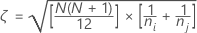
H statistic
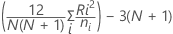
Where 
We will then declare "significance" if:

Where 
Where α is a specified family alpha value, 