What is the Poisson distribution?
The Poisson distribution is specified by one parameter: lambda (λ). This parameter equals the mean and variance. As lambda increases to sufficiently large values, the normal distribution (λ, λ) may be used to approximate the Poisson distribution.
Use the Poisson distribution to describe the number of times an event occurs in a finite observation space. For example, a Poisson distribution can describe the number of defects in the mechanical system of an airplane or the number of calls to a call center in an hour. The Poisson distribution is often used in quality control, reliability/survival studies, and insurance.
- Data are counts of events (nonnegative integers with no upper bound).
- All events are independent.
- Average rate does not change over the period of interest.

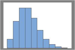
Lambda = 3

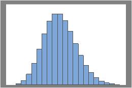
Lambda = 10
What is rate of occurrence?
The rate of occurrence equals the mean (λ) divided by the dimension of your observation space. It is useful for comparing Poisson counts collected in different observation spaces. For example, Switchboard A receives 50 telephone calls in 5 hours, and Switchboard B receives 80 calls in 10 hours. You cannot directly compare these values because their observation spaces are different. You must calculate the occurrence rate to compare these counts. The rate for Switchboard A is (50 calls / 5 hours) = 10 calls/hour. The rate for Switchboard B is (80 calls / 10 hours) = 8 calls/hour.
Differences between the Poisson distribution and the binomial distribution
The Poisson distribution is similar to the binomial distribution because they both model counts of events. However, within its finite observation space, the Poisson distribution places no upper bound on this count: a switchboard could receive an unlimited number of calls in a day and not violate Poisson distribution requirements. Conversely, the binomial distribution does set an upper limit on the count: the number of events you observe cannot be greater than the number of trials you perform.
