Minitab offers several analyses that let you to analyze time series. These analyses include simple forecasting and smoothing methods, correlation analysis methods, and ARIMA modeling. Although correlation analysis can be done separately from ARIMA modeling, Minitab presents the correlation methods as part of ARIMA modeling.
Simple forecasting and smoothing methods
The simple forecasting and smoothing methods model components in a series that is usually easy to observe in a time series plot of the data. This approach decomposes the data into its component parts, and then extends the estimates of the components into the future to provide forecasts. You can choose from the static methods of trend analysis and decomposition, or the dynamic methods of moving average, single and double exponential smoothing, and Winters' method. Static methods have patterns that do not change over time; dynamic methods have patterns that do change over time and estimates are updated using neighboring values.
You can use two methods in combination. That is, you can choose a static method to model one component and a dynamic method to model a different component. For example, you can fit a static trend using trend analysis and dynamically model the seasonal component in the residuals using Winters' method. Or, you can fit a static seasonal model using decomposition and dynamically model the trend component in the residuals using double exponential smoothing. You can also apply a trend analysis and decomposition together so that you can use the wider selection of trend models offered by trend analysis. A disadvantage of combining methods is that the confidence intervals for forecasts are not valid.
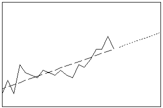
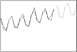
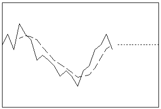
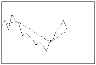
For each of the methods, the following table provides a summary and a graph of fits and forecasts of common data.
Trend Analysis
Fits a general trend model to time series data. Choose between the linear, quadratic, exponential growth or decay, and S-curve trend models. Use this procedure to fit trend when there is no seasonal component in your series.
- Length: long
- Profile: extension of trend line
Decomposition
Separates the times series into linear trend components, seasonal components, and the error. Choose whether the seasonal component is additive or multiplicative with the trend. Use this procedure to forecast when there is a seasonal component in your series or when you want to examine the nature of the component parts.
- Length: long
- Profile: trend with seasonal pattern
Moving Average
Smoothes your data by averaging consecutive observations in a series. You can use this procedure when your data do not have a trend component. If you have a seasonal component, set the length of the moving average to equal the length of the seasonal cycle.
- Length: short
- Profile: flat line
Single Exponential Smoothing
Smoothes your data using the optimal one-step ahead ARIMA (0,1,1) forecasting formula. This procedure works best without a trend or seasonal component. The single dynamic component in a moving average model is the level.
- Length: short
- Profile: flat line
Double Exponential Smoothing
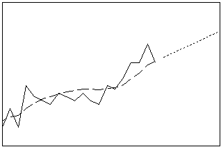
Smoothes your data using the optimal one-step-ahead ARIMA (0,2,2) forecasting formula. This procedure can work well when there is a trend but it can also serve as a general smoothing method. Double Exponential Smoothing calculates dynamic estimates for two components: level and trend.
- Length: short
- Profile: straight line with slope equal to last trend estimate
Winters' Method
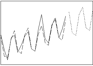
Smoothes your data by Holt-Winters exponential smoothing. Use this procedure when there are trend and seasonality, with these two components being either additive or multiplicative. Winters' Method calculates dynamic estimates for three components: level, trend, and seasonal.
- Length: short to medium
- Profile: trend with seasonal pattern
Correlation analysis and ARIMA modeling
ARIMA (autoregressive integrated moving average) modeling also makes use of patterns in the data, but these patterns might not be easily visible in a plot of the data. Instead, ARIMA modeling uses differencing and the autocorrelation and partial autocorrelation functions to help identify an acceptable model.
ARIMA modeling can be used to model many different time series, with or without trend or seasonal components, and to provide forecasts. The forecast profile depends on the model that is fit. The advantage of ARIMA modeling compared to the simple forecasting and smoothing methods is that it is more flexible in fitting the data. However, identifying and fitting a model can be time-consuming, and ARIMA modeling is not easily automated.
- Differences
- Calculates and stores the differences between data values of a time series. If you want to fit an ARIMA model but your data has a trend or seasonality component, differencing the data is a common step in assessing likely ARIMA models. Differencing is used to simplify the correlation structure and to reveal any underlying pattern.
- Lag
- Calculates and stores the lags of a time series. When you lag a time series, Minitab moves the original values down the column, and inserts missing values at the top of the column. The number of missing values inserted depends on the length of the lag.
- Autocorrelation
- Calculates and creates a graph of the autocorrelations of a time series. Autocorrelation is the correlation between observations of a time series separated by k time units. The plot of autocorrelations is called the autocorrelation function (ACF). View the ACF to guide your choice of terms to include in an ARIMA model.
- Partial Autocorrelation
- Calculates and creates a graph of the partial autocorrelations of a time series. Partial autocorrelations, like autocorrelations, are correlations between sets of ordered data pairs of a time series. As with partial correlations in the regression case, partial autocorrelations measure the strength of relationship with other terms being explained. The partial autocorrelation at a lag of k is the correlation between residuals at time t from an autoregressive model and observations at lag k with terms for all intervening lags in the autoregressive model. The plot of partial autocorrelations is called the partial autocorrelation function (PACF). View the PACF to guide your choice of terms to include in an ARIMA model.
- Cross Correlation
- Calculates and creates a graph of the correlations between two time series.
- ARIMA
- Fits a Box-Jenkins ARIMA model to a time series. In ARIMA, "Autoregressive", "integrated", and "moving average" refer to filtering steps taken in calculating the ARIMA model until only random noise remains. Use ARIMA to model time series behavior and to generate forecasts.
