In This Topic
Multiplicative
Formula
The multiplicative model is:
- Lt = α (Yt / St–p ) + (1 – α) [Lt–1 + Tt–1 ]
- Tt = γ [Lt – Lt–1 ] + (1 – γ) Tt–1
- St = δ (Yt / Lt ) + (1 – δ) St–p
-
 = (Lt–1 + Tt–1 ) St–p
Notation
| Term | Description |
|---|---|
| Lt | level at time t, α is the weight for the level |
| Tt | trend at time t, |
| γ | weight for the trend |
| St | seasonal component at time t |
| δ | weight for the seasonal component |
| p | seasonal period |
| Yt | data value at time t |
 | fitted value, or one-period-ahead forecast, at time t |
Method for calculating initial values for level and trend for multiplicative models
The following method assumes a seasonal length greater than 4.
- Find the mean, minimum, and maximum of the data. For this example:
- Mean = 554.208
- Min = 1
- Max = 1498.47
- For each row of
data, calculate:

- Let N equal the Seasonal length. For this example, N = 12.
- Run regression using the first N "temp values" (calculated
in step 2) as the Y variable, and a vector of 1 through N as the X
variable. So, for this example:
Y X 4104.36 1 4104.36 2 4630.36 3 4922.80 4 4822.40 5 5601.83 6 4891.77 7 4604.44 8 4411.26 9 4123.66 10 4104.36 11 4104.36 12 The slope of the regression line is the initial value for trend.
- Adjust the intercept for the regression
line by subtracting:

The intercept for your data is 4705.24. Subtract 4103.36 from the intercept to obtain an adjusted intercept of 601.879. This adjusted intercept is the initial value for level.
Additive
Formula
- Lt = α (Yt – St–p ) + (1 – α) [Lt–1 + Tt–1 ]
- Tt = γ [Lt – Lt–1 ] + (1 – γ) Tt–1
- St = δ (Yt – Lt ) + (1 – δ) St–p
-
 = Lt–1 + Tt–1 + St–p
Notation
| Term | Description |
|---|---|
| Lt | level at time t, α is the weight for the level |
| Tt | trend at time t, |
| γ | weight for the trend |
| St | seasonal component at time t |
| δ | weight for the seasonal component |
| p | seasonal period |
| Yt | data value at time t |
 | fitted value, or one-period-ahead forecast, at time t |
Method for calculating initial values for level and trend for additive models
The following method assumes a seasonal length greater than 4.
- Let N equal the seasonal length. For this example, N = 12.
- Run regression using the first N data values as the Y variable, and
a vector of 1 through N as the X variable.
So, for this example:
Y X 1.00 1 1.00 2 527.00 3 819.45 4 719.04 5 1498.47 6 788.42 7 501.08 8 307.90 9 20.30 10 1.00 11 1.00 12 The slope of the regression line is the initial value for trend. The intercept of the regression line is the initial value for level.
Method for calculating initial values for seasonal indices for additive models
The following method assumes a seasonal length greater than 4.
- Run regression using the data values as the Y variable, and a
vector of 1 through 24 as the X variable. So, for this example:
Y X 1.00 1 1.00 2 527.00 3 819.45 4 719.04 5 1498.47 6 788.42 7 501.08 8 307.90 9 20.30 10 1.00 11 1.00 12 83.00 13 668.21 14 1121.28 15 1386.84 16 1031.18 17 988.60 18 1380.30 19 1005.97 20 233.69 21 211.87 22 2.00 23 2.40 24 Use the residuals from this regression model in the next step
- Run regression using the residuals as the Y variable, and 12
indicator variables (z.1 through z.12) as the X variables. Fit the
regression model without an intercept (constant) term.
So, for this example:
Residuals z.1 z.2 z.3 z.4 z.5 z.6 z.7 z.8 z.9 z.10 z.11 z.12 -508.261 1 0 0 0 0 0 0 0 0 0 0 0 -512.170 0 1 0 0 0 0 0 0 0 0 0 0 9.926 0 0 1 0 0 0 0 0 0 0 0 0 298.460 0 0 0 1 0 0 0 0 0 0 0 0 194.145 0 0 0 0 1 0 0 0 0 0 0 0 969.667 0 0 0 0 0 1 0 0 0 0 0 0 255.705 0 0 0 0 0 0 1 0 0 0 0 0 -35.538 0 0 0 0 0 0 0 1 0 0 0 0 -232.625 0 0 0 0 0 0 0 0 1 0 0 0 -524.137 0 0 0 0 0 0 0 0 0 1 0 0 -547.346 0 0 0 0 0 0 0 0 0 0 1 0 -551.254 0 0 0 0 0 0 0 0 0 0 0 1 -473.161 1 0 0 0 0 0 0 0 0 0 0 0 108.141 0 1 0 0 0 0 0 0 0 0 0 0 557.303 0 0 1 0 0 0 0 0 0 0 0 0 818.952 0 0 0 1 0 0 0 0 0 0 0 0 459.378 0 0 0 0 1 0 0 0 0 0 0 0 412.890 0 0 0 0 0 1 0 0 0 0 0 0 800.684 0 0 0 0 0 0 1 0 0 0 0 0 422.451 0 0 0 0 0 0 0 1 0 0 0 0 -353.739 0 0 0 0 0 0 0 0 1 0 0 0 -379.468 0 0 0 0 0 0 0 0 0 1 0 0 -593.247 0 0 0 0 0 0 0 0 0 0 1 0 The coefficients from this regression model are the initial values for the seasonal indices. The coefficients are:Period COEF1 1 -490.711 2 -202.014 3 283.615 4 558.706 5 326.762 6 691.278 7 528.195 8 193.456 9 -293.182 10 -451.803 11 -570.297 12 -574.005 Note
The indicator variables z.1 through z.12 indicate which month of the period that each data point belongs to. For example, the variable z.1 is equal to1 for the first month of the period, and it is equal to 0 otherwise.
Model fitting
Winters' method employs a level component, a trend component, and a seasonal component at each period. It uses three weights, or smoothing parameters, to update the components at each period. Initial values for the level and trend components are obtained from a linear regression on time. Initial values for the seasonal component are obtained from a dummy-variable regression using detrended data.
Forecasting
Winters' Method uses the level, trend, and seasonal components to generate forecasts. Winters' Method also uses data up to the forecast origin time to generate the forecasts.
Formula
- Multiplicative method: (Lt + mTt) * St + m −p
- Additive method: Lt + mTt +St + m −p
Notation
| Term | Description |
|---|---|
| Lt | level |
| Tt | trend at time t |
| Term | Description |
|---|---|
| St + m −p | seasonal component for the same period from the previous year |
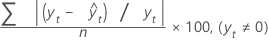
MAPE
Mean absolute percentage error (MAPE) measures the accuracy of fitted time series values. MAPE expresses accuracy as a percentage.
Formula
Notation
| Term | Description |
|---|---|
| yt | actual value at time t |
 | fitted value |
| n | number of observations |
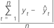
MAD
Mean absolute deviation (MAD) measures the accuracy of fitted time series values. MAD expresses accuracy in the same units as the data, which helps conceptualize the amount of error.
Formula
Notation
| Term | Description |
|---|---|
| yt | actual value at time t |
 | fitted value |
| n | number of observations |
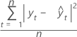
MSD
Mean squared deviation (MSD) is always computed using the same denominator, n, regardless of the model. MSD is a more sensitive measure of an unusually large forecast error than MAD.
Formula
Notation
| Term | Description |
|---|---|
| yt | actual value at time t |
 | fitted value |
| n | number of observations |