A quality engineer at an engine factory wants to perform a test for bimodality on pistons from two suppliers. The engineer measures the lengths of a random sample of 100 pistons from each of the suppliers.
The script uses the diptest package for R to test whether the data are unimodal. If the test rejects the null hypothesis for unimodal data, then the script assumes that the data are a mix of two normal distributions. The script uses the mixtools package for R to display descriptive statistics and density curves for two normal distributions.
- Pass a single column from a Minitab worksheet as input.
- Add a table title.
- Add column labels for a table.
- Send a table to the Minitab Output pane.
- Create a graph and send the graph to the Minitab Output pane.
| File | Description |
|---|---|
| bimodal.R | An R script that takes a column from a Minitab worksheet, tests for unimodality, and produces results for a mix of two normal distributions if the data are not unimodal. |
All the files referenced in this guide are available in this .ZIP file: r_guide_files.zip.
Prerequisites
-
The R script in the below example requires the following R packages:
- mtbr
- The R package that integrates Minitab and R. In the example, functions from this module send R results to Minitab. For information on how to install Minitab's R package, go to Step 2: Install mtbr.
- mixtools
- The R package that the script uses to create output for a mixture of normal distributions.
- diptest
- The R package that the script uses to test whether the data are unimodal.
install.packages("mixtools")For assistance with the installation of R packages, please consult with your organization's technical support department. Minitab Technical Support cannot assist with the installation of R packages.
Steps to run the example
- Ensure you have installed the required modules: mtbr.
- Save the R script file, bimodal.R, to your Minitab default file location. For more information on where Minitab looks for R script files, go to Default folders for R files for Minitab.
- Open the sample data set ProcessEnergyCost.MWX .
-
In the Minitab Command
Line pane, enter
RSCR "bimodal.R" "Process 1". - Select Run.
bimodal.R
# Load the necessary libraries
#Original code by Valentina Tillman
library(mixtools)
library(mtbr)
library(diptest)

# Retrieve sample data
input_column <- commandArgs(trailingOnly = TRUE)
data <- mtb_get_column(input_column)
dip_test_result <- dip.test(data)

if (dip_test_result$p.value < 0.05) {
  # Fit a bimodal mixture model
  bimodal_fit <- normalmixEM(data, k = 2)

  # Manually extract parameter estimates and format them as a data frame
  bimodal_table <- data.frame(
    Mean = bimodal_fit$mu,
    Standard_Deviation = bimodal_fit$sigma,
    Proportion = bimodal_fit$lambda #tells you what % of the data is clustered around which mean. Also called lambda
  )

  # Define title and headers
  mytitle <- "Modeling a Bimodal Distribution"
  myheaders <- names(bimodal_table)

  # Add the table to the mtbr output
  mtb_add_table(columns = bimodal_table, headers = myheaders, title = mytitle)

  png("r_bimodal_image.png")
  plot(bimodal_fit, density = TRUE, which = 2)
  graphics.off()
  mtb_add_image("r_bimodal_image.png")

  # Now generate tolerance intervals using the parameters found using mixtools
  # Set the desired coverage level (e.g., 95%)
  coverage_level <- 0.95
  alpha <- 1 - coverage_level

  # Calculate the tolerance intervals for each component
  tolerance_intervals <- lapply(1:2, function(i) {
    mu <- bimodal_fit$mu[i]
    sigma <- bimodal_fit$sigma[i]
    n <- bimodal_fit$lambda[i]  # proportion of the component

    # Calculate the critical value for the normal distribution
    z <- qnorm(1 - alpha / (2 * n))

    # Calculate lower and upper bounds of the tolerance interval
    lower_bound <- mu - z * sigma
    upper_bound <- mu + z * sigma

    c(lower_bound, upper_bound)
  })

  # Show the tolerance intervals
  tolerance_intervals_df <- data.frame(
    Component = c("First Mode", "Second Mode"),
    Lower_Bound = sapply(tolerance_intervals, "[", 1),
    Upper_Bound = sapply(tolerance_intervals, "[", 2)
  )

  myheaders <- c("Component", "Lower Bound", "Upper Bound")
  mytitle <- "Tolerance Intervals for Bimodal Distribution"
  mtb_add_table(columns = tolerance_intervals_df, headers = myheaders, title = mytitle)


} else {
  mtb_add_message("This data is unimodal.")
}
Results
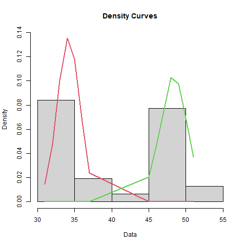
Modeling a Bimodal Distribution
| Mean | Standard_Deviation | Proportion |
|---|---|---|
| 34.1875 | 1.50909 | 0.516129 |
| 48.3333 | 1.84992 | 0.483871 |
Tolerance Intervals for Bimodal Distribution
| Component | Lower Bound | Upper Bound |
|---|---|---|
| First Mode | 31.6821 | 36.6929 |
| Second Mode | 45.3200 | 51.3467 |