In This Topic
- Statistics
- Hypothesis test for a difference in rates for the normal approximation
- Hypothesis test for a difference in rates for the exact method
- Hypothesis test for a difference in rates with the pooled rate method
- Hypothesis test for a difference in means for the normal approximation method
- Hypothesis test for a difference in means for the exact method
- Hypothesis test for a difference in means for the pooled mean method
- Confidence interval for the difference in rates
- Confidence bounds for the difference in rates
- Confidence interval for the difference in means
- Confidence bounds for the difference in means
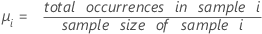
Statistics
| Term | Description |
|---|---|
| rate of occurrence for sample i |
 |
| Term | Description |
|---|---|
| mean number of occurrences in sample i |
 |
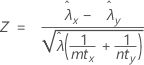
Hypothesis test for a difference in rates for the normal approximation
Formula
The normal approximation test is based on the following Z-statistic, which is approximately distributed as a standard normal distribution under the null hypothesis:
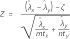
Minitab uses the following p-value equations for the respective alternative hypotheses:


Notation
| Term | Description |
|---|---|
 | observed value of rate for sample X |
 | observed value of rate for sample Y |
| ζ | true value of the difference between the population rates of two samples |
| ζ0 | hypothesized value of the difference between the population rates of two samples |
| m | sample size of sample X |
| n | sample size of sample Y |
| tx | length of sample X |
| ty | length of sample Y |
Hypothesis test for a difference in rates for the exact method
Formula
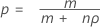
When the hypothesized difference equals 0, Minitab uses an exact procedure to test the following null hypothesis:
H0: ζ = λx – λy = 0, or H0: λx = λy
The exact procedure is based on the following fact, assuming the null hypothesis is true:
S | W ~ Binomial(w, p)
where:


W = S + U

-
H1: ζ > 0: p-value = P(S ≥ s | w = s + u, p = p0)
-
H1: ζ < 0: p-value = P(S ≤ s | w = s + u, p = p0)
- H1: ζ ≠ 0:
- if P(S ≤ s | w = s + u, p = p0) ≤ 0.5 or P(S ≥ s | w = s + u, p = p0) ≤ 0.5
then the p-value = 2 × min {P(S ≤ s | w = s + u, p = p0), P(S ≥ s | w = s + u, p = p0)}
- otherwise, p-value = 1.0
- if P(S ≤ s | w = s + u, p = p0) ≤ 0.5 or P(S ≥ s | w = s + u, p = p0) ≤ 0.5
where:

Notation
| Term | Description |
|---|---|
 | observed value of the rate for sample X |
 | observed value of the rate for sample Y |
| λx | true value of the rate for population X |
| λy | true value of rate for population Y |
| ζ | true value of the difference between the population rates of two samples |
| tx | length of sample X |
| ty | length of sample Y |
| m | sample size of sample X |
| n | sample size of sample Y |
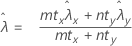
Hypothesis test for a difference in rates with the pooled rate method
When you test a zero difference with the following null hypothesis, you have the option to use a pooled rate for both samples:

Formula
The pooled-rate procedure is based on the following Z-statistic, which is approximately distributed as a standard normal distribution under the following null hypothesis:
where:
Minitab uses the following p-value equations for the respective alternative hypotheses:


Notation
| Term | Description |
|---|---|
 | observed value of the rate for sample X |
 | observed value of the rate for sample Y |
| λx | true value of the rate for population X |
| λy | true value of the rate for population Y |
| ζ | true value of the difference between the population rates of two samples |
| m | sample size of sample X |
| n | sample size of sample Y |
| tx | length of sample X |
| ty | length of sample Y |
Hypothesis test for a difference in means for the normal approximation method
Formula
The normal approximation test is based on the following Z-statistic, which is approximately distributed as a standard normal distribution under the null hypothesis.
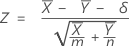
Minitab uses the following p-value equations for the respective alternative hypotheses:


Notation
| Term | Description |
|---|---|
 | observed value of the mean number of occurrences in sample X |
 | observed value of the mean number of occurrences in sample Y |
| δ | true value of the difference between the population means of two sample |
| δ 0 | hypothesized value of the difference between the population means of two samples |
| m | sample size of sample X |
| n | sample size of sample Y |
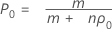
Hypothesis test for a difference in means for the exact method
Formula

The exact procedure is based on the following fact, assuming the null hypothesis is true:
S | W ~ Binomial(w, p)
where:


W = S + U
Minitab uses the following p-value equations for the respective alternative hypotheses:
H1: δ > 0: p-value = P(S ≥ s | w = s + u, δ = 0)
H1: δ < 0: p-value = P(S ≤ s | w = s + u, δ = 0)
-
if P(S ≤ s|w = s + u, δ = 0) ≤ 0.5
or P(S ≥ s|w = s + u, δ = 0) ≤ 0.5
then:

- otherwise, p-value = 1.0
A two-tailed test is not an equal-tailed test unless m = n.
Notation
| Term | Description |
|---|---|
| μx | true value of the mean number of occurrences in population X |
| μy | true value of the mean number of occurrences in population Y |
| δ | true value of the difference between the population means of two samples |
| m | sample size of sample X |
| n | sample size of sample Y |
Hypothesis test for a difference in means for the pooled mean method
Formula

The pooled-mean procedure is based on the following Z-value, which is approximately distributed as a standard normal distribution under the following null hypothesis:
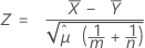
where:
Minitab uses the following p-value equations for the respective alternative hypotheses:


Notation
| Term | Description |
|---|---|
 | observed value of the mean number of occurrences in sample X |
 | observed value of the mean number of occurrences in sample Y |
| µx | true value of the mean number of occurrences in population X |
| µy | true value of the mean number of occurrences in population Y |
| δ | true value of the difference between the population means of two samples |
| m | sample size of sample X |
| n | sample size of sample Y |
Confidence interval for the difference in rates
Formula
A 100(1 – α)% confidence interval for the difference between two population Poisson rates is given by:
Notation
| Term | Description |
|---|---|
 | observed value of rate for sample X |
 | observed value of rate for sample Y |
| ζ | true value of the difference between the population rates of two samples |
| zx | upper x percentile point of the standard normal distribution, where 0 < x < 1 |
| m | sample size of sample X |
| n | sample size of sample Y |
| tx | length of sample X |
| ty | length of sample Y |
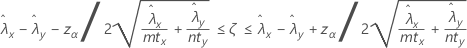
Confidence bounds for the difference in rates
Formula
When you specify a "greater than" test, a 100(1 – α)% lower confidence bound for the difference between two population Poisson rates is given by:
When you specify a "less than" test, a 100(1 – α)% upper confidence bound for the difference between two population Poisson rates is given by:
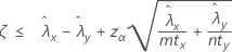
Notation
| Term | Description |
|---|---|
 | observed value of rate for sample X |
 | observed value of rate for sample Y |
| ζ | true value of the difference between the population rates of two samples |
| zx | the upper x percentile point on the standard normal distribution, where 0 < x < 1 |
| m | sample size of sample X |
| n | Sample size of sample Y |
| tx | length of sample X |
| ty | length of sample Y |
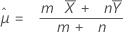
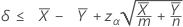
Confidence interval for the difference in means
Formula
A 100(1 – α)% confidence interval for the difference between two population Poisson means is given by:

Notation
| Term | Description |
|---|---|
 | observed value of the mean number of occurrences in sample X |
 | observed value of the mean number of occurrences in sample Y |
| δ | true value of the difference between the population means of two samples |
| zx | upper x percentile point on the standard normal distribution, where 0 < x < 1 |
| m | sample size of sample X |
| n | sample size of sample Y |
Confidence bounds for the difference in means
Formula
When you specify a "greater than" test, a 100(1 – α)% lower confidence bound for the difference between two population Poisson means is given by:

When you specify a "less than" test, a 100(1 – α)% upper confidence bound for the difference between two population Poisson means is given by:
Notation
| Term | Description |
|---|---|
 | observed value of the mean number of occurrences in sample X |
 | observed value of the mean number of occurrences in sample Y |
| δ | true value of the difference between the population means of two samples |
| zx | upper x percentile point on the standard normal distribution, where 0 < x < 1 |
| m | sample size of sample X |
| n | sample size of sample Y |