In This Topic
Single exponential smoothing
The smoothed values are obtained in one of two ways: with an optimal weight generated by Minitab or a weight that you specify.
Optimal ARIMA weight
- Minitab fits with an ARIMA (0,1,1) model with no constant and stores the fits.
- The initial smoothed value for the Single Exponential Smoothing analysis is the first non-missing fit from the ARIMA model.
- Since the fits are lagged one time unit, Minitab uses
backcasting to calculate the initial fitted value (at time one):
- initial fitted value = [the first smoothed value – α (first data value)] / (1 – α)
Notation
| Term | Description |
|---|---|
| 1 – α | Estimates the MA parameter where α is the smoothing constant. |
Specified weight
- Minitab uses the average of the first six (or N, if N < 6) observations for the initial smoothed value (at time zero). Equivalently, Minitab uses the average of the first six (or N, if N < 6) observations for the initial fitted value (at time one). Fit(i) = Smoothed(i – 1).
- Subsequent smoothed values are calculated from the formula:
- smoothed value at time t = α (data at t) + (1 – α) (smoothed value at time t – 1)
Notation
| Term | Description |
|---|---|
| α | weight |
Forecasts
The fitted value at time t is the smoothed value at time t – 1. The forecasts are the fitted value at the forecast origin. If you forecast 10 time units ahead, the forecasted value for each time will be the fitted value at the origin. Data up to the origin are used for the smoothing.
In naive forecasting, the forecast for time t is the data value at time t – 1. Perform single exponential smoothing with a weight of one to perform naive forecasting.
Prediction limits
Formula
- Upper limit = Forecast + 1.96 × 1.25 × MAD
- Lower limit = Forecast – 1.96 × 1.25 × MAD
The value of 1.25 is an approximate proportionality constant of the standard deviation to the mean absolute deviation. Hence, 1.25 × MAD is approximately the standard deviation.
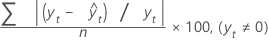
MAPE
Mean absolute percentage error (MAPE) measures the accuracy of fitted time series values. MAPE expresses accuracy as a percentage.
Formula
Notation
| Term | Description |
|---|---|
| yt | actual value at time t |
 | fitted value |
| n | number of observations |
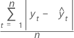
MAD
Mean absolute deviation (MAD) measures the accuracy of fitted time series values. MAD expresses accuracy in the same units as the data, which helps conceptualize the amount of error.
Formula
Notation
| Term | Description |
|---|---|
| yt | actual value at time t |
 | fitted value |
| n | number of observations |
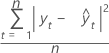
MSD
Mean squared deviation (MSD) is always computed using the same denominator, n, regardless of the model. MSD is a more sensitive measure of an unusually large forecast error than MAD.
Formula
Notation
| Term | Description |
|---|---|
| yt | actual value at time t |
 | fitted value |
| n | number of observations |