Follow the steps appropriate for the models that you want to evaluate.
The steps are the same for seasonal and non-seasonal models but details differ.
Fit a non-seasonal ARIMA model
Complete the following steps to specify the column of data that you want to analyze with a non-seasonal ARIMA model. When you fit models with a constant term, candidate models have p + q ≤ 9. When you fit models without a constant term, candidate models have p + q ≤ 10. Candidate models with d = 2 are fit without a constant term.
Pre-requisites
Usually, you evaluate the need for a transformation and determine the differencing order before you begin this analysis.
Transformation
Use a time series plot to determine if the variance of a time series is
stationary. If the time series has a pattern in the spread of the points, then
the variance is not stationary. Use a Box-Cox transformation of a time series to try to make the variance of
the series stationary. To evaluate a Box-Cox transformation for a time series, choose
Stat > Time Series > Box-Cox Transformation. For information on the use of a Box-Cox transformation in Forecast with
Best ARIMA Model, go to Select the analysis options for Forecast with Best ARIMA Model.
Differencing
Examine a plot of the autocorrelation function (ACF) for a series to determine the order of differencing. The usual pattern on an ACF plot that shows a need for differencing is a trend that decreases slowly. If the data support further differencing, the same pattern occurs in the ACF of the differenced data. To perform an autocorrelation analysis, choose Stat > Time Series > Autocorrelation. Also consider the augmented Dickey-Fuller test to determine the order. Specify the differencing order when you evaluate the models.
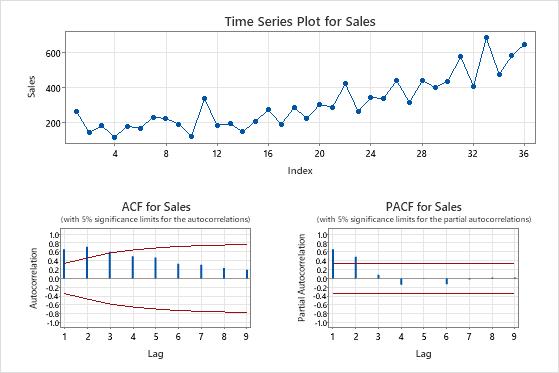
ACF plot of a time series with a trend
In these results, the time
series plot of the original data shows a clear trend. The time series plot of
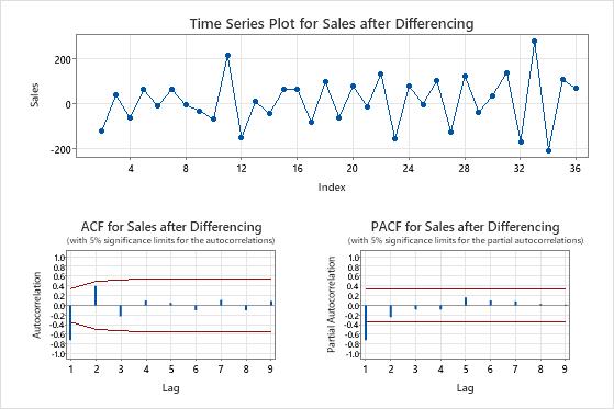
the differenced data shows the differences between consecutive values. The differenced data appear stationary
because the points follow a horizontal path without obvious patterns in the
variation.
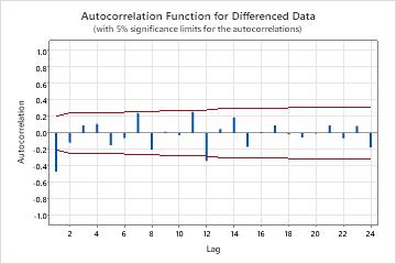
The ACF plots also show the effect of differencing. In these results, the ACF plot of the
original data shows slowly-decreased spikes across lags. This pattern indicates that
the data are not stationary. In the ACF plot of the differenced data, the only spike that is significantly different from 0 is at lag 1.
Evaluate non-seasonal models
In Series, enter a column of numeric data that were collected at regular intervals and recorded in time order.
In Differencing order d, choose the order for nonseasonal differencing.
For Autoregressive order p, choose a minimum value to evaluate and a maximum value to evaluate. The analysis fits models with all the combinations of autoregressive and moving average orders in the choices. If you enter the same value for the minimum and the maximum, then the analysis uses that value for all the candidate models.
For Moving average order q, choose a minimum value to evaluate and a maximum value to evaluate. The analysis fits models with all the combinations of autoregressive and moving average orders in the choices. If you enter the same value for the minimum and the maximum, then the analysis uses that value for all the candidate models.
Select Include the constant term in models to include the constant term in the model. With a constant term, the model can estimate a series where the mean is not 0. Without a constant term, the mean of the series that the model fits is 0. If the analysis cannot fit a model with a constant term, then the analysis tries to fit the model without the constant term.
In Number of forecasts, enter the number of consecutive time periods that you want forecasts for. Usually, you enter the minimum number to provide the forecast that you want. For example, if you have monthly data and want to get a forecast for 6 months past the end of the series, enter 6.
Choose Forecast from the end of the series or Forecast from the Kth value in the series. If you enter a value, Minitab uses only the data up to that row number for the forecasts. The forecast values differ from the fits because Minitab uses all the data to calculate the fits. For example, an analyst has 5 years of monthly data for January through December. The analyst wants to generate a forecast for the next month, but the final month of December's data are incomplete. The analyst specifies to forecast from the 59th value in the series and specifies two forecasts. The analysis uses the data through the first 59 months to generate forecasts for December and January.
Before you use an ARIMA model to forecast, verify that the model fits the data well. Examine residual diagnostics to determine whether the model meets the assumptions for an ARIMA model. For more information, go to Interpret the key results for Forecast with Best ARIMA Model.
Fit a seasonal ARIMA model
Complete the following steps to specify the column of data that you want to analyze with a seasonal ARIMA model. When you fit models with a constant term, candidate models have p + q + P + Q ≤ 9. When you fit models without a constant term, candidate models have p + q + P + Q ≤ 10. Candidate models with d + D > 1 are fit without a constant term.
Pre-requisites
Usually, you evaluate the need for a transformation and determine the differencing order before you begin this analysis.
Transformation
Use a time series plot to determine if the variance of a time series is
stationary. If the time series has a pattern in the spread of the points, then
the variance is not stationary. Use a Box-Cox transformation of a time series to try to make the variance of
the series stationary. To evaluate a Box-Cox transformation for a time series, choose
Stat > Time Series > Box-Cox Transformation. For information on the use of a Box-Cox transformation in Forecast with
Best ARIMA Model, go to Select the analysis options for Forecast with Best ARIMA Model.
Differencing
Examine a plot of the autocorrelation function (ACF) for a series to determine the non-seasonal and seasonal orders of differencing. A seasonal pattern that repeats each kth period of time indicates that you should take the kth difference to remove a portion of the pattern. A trend that decreases slowly indicates that you should also use a non-seasonal difference. If the data support further differencing, the same patterns occur in the ACF of the differenced data. Orders of seasonal differencing greater than 1 are rare. To perform an autocorrelation analysis, choose Stat > Time Series > Autocorrelation. Specify differencing orders when you evaluate the models.
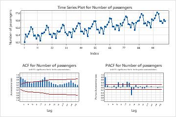
ACF plot of a time series with a trend and a seasonal pattern
In these results, the time
series plot of the original data shows an upwards trend and a seasonal pattern with a period of 12. The time series plot of
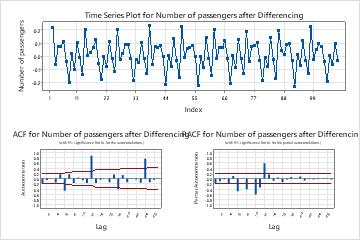
the differenced data shows the differences between consecutive values.
The ACF plot for the data after differncing shows the effect of non-seasonal differencing. In these results, the ACF plot of the
original data shows slowly-decreased spikes across lags. Spikes also appear at the seasonal lags. These two patterns indicate that
the data are not stationary. In the ACF plot of the data after non-seasonal differencing, the significant spikes are at the seasonal lags.
The ACF plot of the data after a seasonal difference and a non-seasonal difference does not show the seasonal pattern. the orders of differencing appropriate for these data are 1 non-seasonal difference and 1 seasonal difference.
Evaluate seasonal models
In Series, enter a column of numeric data that were collected at regular intervals and recorded in time order.
In Differencing order d, choose the order for nonseasonal differencing.
For Autoregressive order p, choose a minimum value to evaluate and a maximum value to evaluate. The analysis fits models with all the combinations of autoregressive and moving average orders in the choices. If you enter the same value for the minimum and the maximum, then the analysis uses that value for all the candidate models.
For Moving average order q, choose a minimum value to evaluate and a maximum value to evaluate. The analysis fits models with all the combinations of autoregressive and moving average orders in the choices. If you enter the same value for the minimum and the maximum, then the analysis uses that value for all the candidate models.
Select Fit seasonal models with period and enter the length of the seasonal pattern. For example, if you collect data monthly and the data have a yearly pattern, enter 12.
In Seasonal differencing order D, choose the order for seasonal differencing. Most series with a seasonal pattern use a seasonal order of differencing to make the data stationary. 1 is sufficient for most seasonal patterns.
For Autoregressive order P, choose a minimum value to evaluate and a maximum value to evaluate. The analysis fits models with all the combinations of autoregressive and moving average orders in the choices. If you enter the same value for the minimum and the maximum, then the analysis uses that value for all the candidate models.
For Moving average order Q, choose a minimum value to evaluate and a maximum value to evaluate. The analysis fits models with all the combinations of autoregressive and moving average orders in the choices. If you enter the same value for the minimum and the maximum, then the analysis uses that value for all the candidate models.
Select Include the constant term in models to include the constant term in the model. With a constant term, the model can estimate a series where the mean is not 0. Without a constant term, the mean of the series that the model fits is 0. If the analysis cannot fit a model with a constant term, then the analysis tries to fit the model without the constant term.
In Number of forecasts, enter the number of consecutive time periods that you want forecasts for. Usually, you enter the minimum number to provide the forecast that you want. For example, if you have monthly data and want to get a forecast for 6 months past the end of the series, enter 6.
Choose Forecast from the end of the series or Forecast from the Kth value in the series. If you enter a value, Minitab uses only the data up to that row number for the forecasts. The forecast values differ from the fits because Minitab uses all the data to calculate the fits. For example, an analyst has 5 years of monthly data for January through December. The analyst wants to generate a forecast for the next month, but the final month of December's data are incomplete. The analyst specifies to forecast from the 59th value in the series and specifies two forecasts. The analysis uses the data through the first 59 months to generate forecasts for December and January.
Before you use an ARIMA model to forecast, verify that the model fits the data well. Examine residual diagnostics to determine whether the model meets the assumptions for an ARIMA model. For more information, go to Interpret the key results for Forecast with Best ARIMA Model.