Interpret the key results for Forecast with Best ARIMA Model

Complete the following steps to interpret the model selection process and the results for the ARIMA analysis. Key output includes the model-selection statistics, p-value, coefficients, Ljung-Box chi-square statistics, and the autocorrelation function of the residuals.

In This Topic

Step 1: Consider alternative models
Step 2: Determine whether each term in the model is significant
Step 3: Determine whether your model meets the assumptions of the analysis

Step 1: Consider alternative models

The Model Selection table displays the criteria for each model in the search. The table displays the order of the terms where p is the autoregressive term, d is the differencing term, and q is the moving average term. Seasonal terms use upper-case letters and non-seasonal terms use lower-case letters.

Use AIC, AICc and BIC to compare different models. Smaller values are desirable. However, the model with the least value for a set of terms does not necessarily fit the data well. Use tests and plots to assess how well the model fits the data. By default, the ARIMA results are for the model with the best value of AICc.

Select Select an Alternative Model to open a dialog that includes a the Model Selection table. Compare the criteria to investigate models with similar performance.

Use the ARIMA output to verify that the terms in the model are statistically significant and that the model meets the assumptions of the analysis. If none of the models in the table fit the data well, consider models with different orders of differencing.

Also consider an alternative model when an alternative model performs almost as well as the best model and has lower orders for the autoregressive and moving average terms. A model with fewer terms is easier to interpret and can have better forecasting ability. Models with fewer terms are also less likely to include redundant terms. For example, seasonal autoregressive terms are sometimes redundant with seasonal moving average terms. Redundant terms sometimes make the estimates of the coefficients unstable. The following are some of the consequences of unstable coefficients:

Coefficients can seem to be insignificant even when a significant relationship exists between the predictor and the response.
Coefficients for highly correlated predictors will vary widely from sample to sample.
Removing any highly correlated terms from the model will greatly affect the estimated coefficients of the other highly correlated terms. Coefficients of the highly correlated terms can even have the wrong sign.

* WARNING * Inestimable ARIMA(p, d, q) models that do not include a constant term:
(2, 1, 2)

Model Selection

Model (d = 1)	LogLikelihood	AICc	AIC	BIC
p = 0, q = 2*	-197.052	400.878	400.103	404.769
p = 1, q = 2	-196.989	403.311	401.978	408.199
p = 1, q = 0	-201.327	407.029	406.654	409.765
p = 2, q = 0	-200.239	407.251	406.477	411.143
p = 1, q = 1	-200.440	407.655	406.880	411.546
p = 2, q = 1	-201.776	412.884	411.551	417.773
p = 0, q = 1	-204.584	413.542	413.167	416.278
p = 0, q = 0	-213.614	429.350	429.229	430.784

Key results: AICc, BIC, and AIC

The ARIMA(0, 1, 2) has the best value of AICc. The ARIMA results that follow are for the ARIMA(0, 1, 2) model. If the model does not fit the data well enough, consider other models with similar performance, such as the ARIMA(1, 1, 2) model and the ARIMA (1, 1, 1) model. If none of the models fit the data well enough, consider whether to use a different type of model.

Step 2: Determine whether each term in the model is significant

To determine whether the association between the response and each term in the model is statistically significant, compare the p-value for the term to your significance level to assess the null hypothesis. The null hypothesis is that the term is not significantly different from 0, which indicates that no association exists between the term and the response. Usually, a significance level (denoted as α or alpha) of 0.05 works well. A significance level of 0.05 indicates a 5% risk of concluding that the term is not significantly different from 0 when it is significantly different from 0.

P-value ≤ α: The term is statistically significant: If the p-value is less than or equal to the significance level, you can conclude that the coefficient is statistically significant.
P-value > α: The term is not statistically significant: If the p-value is greater than the significance level, you cannot conclude that the coefficient is statistically significant. You may want to refit the model without the term.

Final Estimates of Parameters

Type	Coef	SE Coef	T-Value	P-Value
AR 1	-0.504	0.114	-4.42	0.000
Constant	150.415	0.325	463.34	0.000
Mean	100.000	0.216

Key Results: P, Coef

The autoregressive term has a p-value that is less than the significance level of 0.05. You can conclude that the coefficient for the autoregressive term is statistically significant, and you should keep the term in the model.

Step 3: Determine whether your model meets the assumptions of the analysis

Use the Ljung-Box chi-square statistics, the autocorrelation function (ACF) of the residuals, and the partial autocorrelation function (PACF) of the residuals to determine whether the model meets the assumptions that the residuals are independent. If the assumption is not met, the model may not fit the data and you should use caution when you interpret the results or consider other models.

Ljung-Box chi-square statistics: To determine whether the residuals are independent, compare the p-value to the significance level for each chi square statistic. Usually, a significance level (denoted as α or alpha) of 0.05 works well. If the p-value is greater than the significance level, you can conclude that the residuals are independent and that the model meets the assumption.
Autocorrelation function of the residuals: If no significant correlations are present, you can conclude that the residuals are independent. However, you may see 1 or 2 significant correlations at higher order lags that are not seasonal lags. These correlations are usually caused by random error instead and are not a sign that the assumption is not met. In this case, you can conclude that the residuals are independent.
Partial autocorrelation function of the residuals: If no significant correlations are present, you can conclude that the residuals are independent. However, you may see 1 or 2 significant correlations at higher order lags that are not seasonal lags. These correlations are usually caused by random error instead and are not a sign that the assumption is not met. In this case, you can conclude that the residuals are independent.

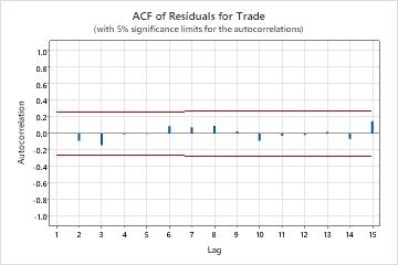
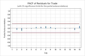
Key Results: P-Value, ACF of Residuals, PACF of residuals
In these results, the p-values for the Ljung-Box chi-square statistics are all greater than 0.05. None of the correlations for the autocorrelation function of the residuals or the partial autocorrelation function of the residuals are significant. You can conclude that the model meets the assumption that the residuals are independent.

Lag	12	24	36	48
Chi-Square	4.05	12.13	25.62	32.09
DF	10	22	34	46
P-Value	0.945	0.955	0.849	0.940