Example of Forecast with Best ARIMA Model for a seasonal model

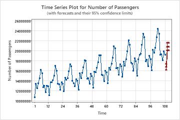
An analyst collected data on the number of airline passengers for 108 months. The analyst wants to use an ARIMA model to generate forecasts for the data. The analyst previously examined a time series plot of the data and observed that the variation in the seasonal cycle increases over time. The analyst concluded that a natural log transformation of the data is appropriate. After the transformation, the analyst examined the time series plot of the transformed data and the autocorrelation function (ACF) plot of the transformed data. Both plots suggest that the starting point for the model is to choose 1 for the order of non-seasonal differencing and 1 for the order of seasonal differencing. The analyst requests forecasts for the next 3 months.

  1. Open the sample data AirPassengers.mtw.
  2. Choose Stat > Time Series > Forecast with Best ARIMA Model.
  3. In Series, enter Number of Passengers.
  4. In Differencing order d, select 1.
  5. Select Fit seasonal models with period and enter 12 for the period.
  6. In Seasonal differencing order D, select 1.
  7. In Number of forecasts, enter 3.
  8. Select Options.
  9. In Box-Cox Transformation, select λ = 0 (natural log).
  10. Select OK in each dialog box.

Interpret the results

The model selection table ranks the models from the search in order by AICc. The ARIMA(0, 1, 1)(1, 1, 0) model has the least AICc. The ARIMA results that follow are for the ARIMA(0, 1, 1)(1, 1, 0) model.

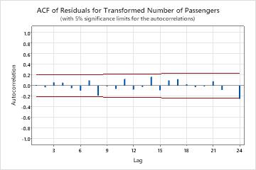
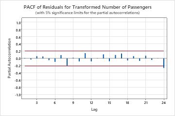
The p-values in the parameters table show that the model terms are significant at the 0.05 level. The analyst concludes that the coefficients belong in the model. The p-values for the Modified Box-Pierce (Ljung-Box) statistics are all insignificant at the 0.05 level. The ACF of the residuals and the PACF of the residuals show a spike at lag 24. Because a large spike at a high lag number is usually a false positive and the test statistics are all insignificant, the analyst concludes that the model meets the assumption that the residuals are independent. The analyst concludes that examination of the forecasts is reasonable.

* WARNING * Inestimable ARIMA(p, d, q)(P, D, Q) models that do not include a constant term:
(2, 1, 1)(1, 1, 1)

Method

Seasonal period12
Criterion for best modelMinimum AICc
Box-Cox transformation 
    User-specified λ0
    Transformed series = ln(Number of Passengers) 
Rows used108
Rows unused0

Model Selection

Model (d = 1, D = 1)LogLikelihoodAICcAICBIC
p = 0, q = 1, P = 1, Q = 0*243.477-480.690-480.954-473.292
p = 2, q = 0, P = 0, Q = 1243.903-479.362-479.806-469.590
p = 1, q = 1, P = 1, Q = 0243.496-478.547-478.992-468.776
p = 0, q = 2, P = 1, Q = 0243.480-478.516-478.961-468.745
p = 2, q = 0, P = 1, Q = 1244.424-478.174-478.848-466.079
p = 0, q = 1, P = 0, Q = 0237.930-471.729-471.859-466.752
p = 1, q = 2, P = 0, Q = 0239.930-471.415-471.859-461.644
p = 1, q = 1, P = 0, Q = 0237.929-469.594-469.858-462.196
p = 0, q = 2, P = 0, Q = 0237.924-469.584-469.848-462.186
p = 1, q = 0, P = 0, Q = 1237.442-468.619-468.883-461.221
p = 1, q = 0, P = 1, Q = 1237.551-466.658-467.102-456.887
p = 2, q = 2, P = 0, Q = 0238.267-465.860-466.534-453.765
p = 2, q = 0, P = 0, Q = 0232.478-458.693-458.957-451.295
p = 0, q = 0, P = 0, Q = 1226.062-447.993-448.124-443.016
p = 0, q = 0, P = 1, Q = 1226.282-446.300-446.563-438.902
p = 2, q = 1, P = 0, Q = 0226.105-443.766-444.211-433.995
p = 1, q = 0, P = 0, Q = 0222.409-440.687-440.818-435.710
p = 2, q = 0, P = 1, Q = 0220.456-432.467-432.911-422.696
p = 0, q = 0, P = 1, Q = 0218.236-432.342-432.472-427.364
p = 1, q = 2, P = 1, Q = 1220.708-428.461-429.416-414.092
p = 0, q = 2, P = 0, Q = 1215.116-421.787-422.232-412.016
p = 0, q = 1, P = 0, Q = 1213.007-419.751-420.015-412.353
p = 2, q = 1, P = 0, Q = 1214.469-418.265-418.939-406.169
p = 1, q = 0, P = 1, Q = 0211.232-416.199-416.463-408.801
p = 2, q = 2, P = 0, Q = 1213.877-414.799-415.754-400.431
p = 2, q = 2, P = 1, Q = 1214.698-414.109-415.397-397.520
p = 1, q = 2, P = 0, Q = 1211.492-412.310-412.984-400.215
p = 1, q = 1, P = 0, Q = 1208.149-407.854-408.299-398.083
p = 0, q = 1, P = 1, Q = 1204.745-401.046-401.490-391.275
p = 0, q = 2, P = 1, Q = 1203.978-397.282-397.956-385.187
p = 1, q = 1, P = 1, Q = 1203.564-396.453-397.127-384.358
p = 1, q = 2, P = 1, Q = 0170.812-330.950-331.624-318.855
p = 2, q = 2, P = 1, Q = 0167.845-322.735-323.690-308.367
p = 2, q = 1, P = 1, Q = 0-202.538415.751415.076427.846
* Best model with minimum AICc.  Output for the best model follows.

Final Estimates of Parameters

TypeCoefSE CoefT-ValueP-Value
SAR  12-0.4030.103-3.920.000
MA   10.87040.051017.080.000
Differencing: 1 Regular, 1 Seasonal of order 12
Number of observations after differencing: 95

Model Summary

DFSSMSMSDAICcAICBIC
930.03113260.00033480.0003277-480.690-480.954-473.292
MS = variance of the white noise series

Modified Box-Pierce (Ljung-Box) Chi-Square Statistic

Lag12243648
Chi-Square9.4726.4433.9950.66
DF10223446
P-Value0.4890.2330.4680.295
* WARNING * Inestimable ARIMA(p, d, q)(P, D, Q) models that do not include a constant term:
(2, 1, 1)(1, 1, 1)

Original Series


95% Limits
Time PeriodForecastLowerUpperActual
109168226641622724217434097 
110208238762008075121587153 
111208267022007744321596450 

Transformed Series


95% Limits
Time PeriodForecastSE ForecastLowerUpperActual
10916.63810.018296416.602216.6739 
11016.85140.018449516.815316.8876 
11116.85160.018601416.815116.8880