A marketing analyst wants to use an ARIMA model to generate short-term forecasts for sales of
a shampoo product. The analyst collects sales data from the previous three years.
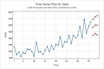
The analyst previously examined a time series plot and the autocorrelation function
(ACF) plot for the series. Both plots suggest 1 as the starting point for the order
of non-seasonal differencing. The data do not exhibit a seasonal pattern on a time
series plot, so the analyst chooses to begin with a nonseasonal model. The analyst
requests forecasts for the next 3 months.
Choose Stat > Time Series > Forecast with Best ARIMA Model.
In Series, enter Sales.
In Differencing order d, select
1.
Deselect Include the constant term in models.
In Number of forecasts, enter
3.
Select OK.
Interpret the results
The model selection table ranks the models from the search in order by AICc. The ARIMA (0, 1, 2)
model has the least AICc. The ARIMA results that follow are for the ARIMA (0, 1, 2)
model.
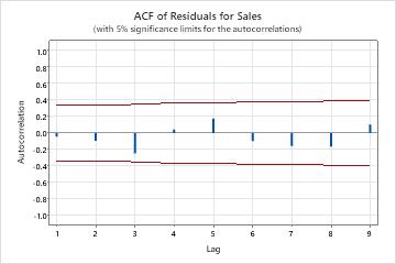
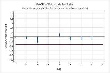
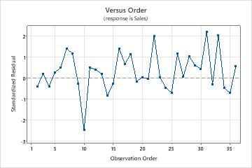
The p-values in the parameters table show that the moving average terms are significant at the 0.05 level. The analyst concludes that the coefficients belong in the model. The p-values for the Modified Box-Pierce (Ljung-Box) statistics are all insignificant at the 0.05 level. The ACF of the residuals and the PACF of the residuals are all within the 0.05 limits on their respective plots. The analyst concludes that the model meets the assumption that the residuals are independent. The analyst concludes that examination of the forecasts is reasonable.
* WARNING * Inestimable ARIMA(p, d, q) models that do not include a constant term: (2, 1, 2)