In This Topic
Model equation
Double exponential smoothing employs a level component and a trend component at each period. Double exponential smoothing uses two weights, (also called smoothing parameters), to update the components at each period. The double exponential smoothing equations are as follows:
Formula
Lt = α Yt + (1 – α) [Lt –1 + Tt –1]
Tt = γ [Lt – Lt –1] + (1 – γ) Tt –1
 = Lt−1
+ Tt−1
= Lt−1
+ Tt−1
If the first observation is numbered one, then level and trend estimates at time zero must be initialized in order to proceed. The initialization method used to determine how the smoothed values are obtained in one of two ways: with optimal weights or with specified weights.
Notation
| Term | Description |
|---|---|
| Lt | level at time t |
| α | weight for the level |
| Tt | trend at time t |
| γ | weight for the trend |
| Yt | data value at time t |
 | predicted value for time t |
Weights
Optimal ARIMA weights
- Minitab fits with an ARIMA (0,2,2) model to the data, in order to minimize the sum of squared errors.
- The trend and level components are then initialized by backcasting.
Specified weights
- Minitab fits a linear regression model to time series data (y variable) versus time (x variable).
- The constant from this regression is the initial estimate of the level component, the slope coefficient is the initial estimate of the trend component.
When you specify weights that correspond to an equal-root ARIMA (0, 2, 2) model, Holt's method specializes to Brown's method1.
Method for calculating initial values for level and trend
can store estimates for level and trend. Minitab uses one of the following methods to calculate the values in the first row of these columns, depending on the options you specify in the dialog box.
If you choose the option Optimal ARIMA in Double Exp Smoothing, then Minitab uses the following method to calculate the first values of level and trend. You can perform these steps by hand.
- Choose to calculate optimal weight values using ARIMA. Complete the dialog box as follows:
- In Autoregressive, enter 0.
- In Difference, enter 2.
- In Moving average, enter 2.
- Uncheck Include constant term in model.
- Click Storage and check Residuals. Click OK in each dialog box.
- Minitab uses the MA values from the ARIMA output to
calculate the optimal weights as follows:

- Then, Minitab calculates back to the initial observation, using
data from later observations:
where:
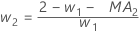
Term Description pi the predicted value of the ith smoothed observation xi the value of the ith observation in the time series ei the value of the ith residual, stored from ARIMA above - Minitab calculates the initial value for level (L1):
- Minitab calculates the initial value for trend (T1):


- Create a column of time indices equal to the length of your column of time series data. A column of integers from 1 to n is sufficient.
- Choose .
- In Responses, enter the column of time series data. In Continuous predictors, enter the column of time indices.
- Click Storage and check Coefficients. Click OK in each dialog box.
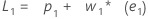
- The initial value for level is:
- The initial value for trend is:
 where:
Term Description L1 initial value for level x1 the value of the first observation in the time series T1 initial value for trend wL the weight value for level wT the weight value for trend β0 the coefficient of the constant term in the regression model β1 the coefficient for the predictor term in the regression model
Forecasts
Double exponential smoothing uses the level and trend components to generate forecasts. The forecast for m periods ahead from a point at time t is as follows:
Formula
Lt + mTt
Data up to the forecast origin time are used for the smoothing.
Notation
| Term | Description |
|---|---|
| Lt | level at time t |
| Tt | trend at time t |
Prediction limits
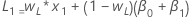
Formula
- Upper limit = Forecast + 1.96 × dt × MAD
- Lower limit = Forecast – 1.96 × dt × MAD
Notation
| Term | Description |
|---|---|
| β | max{α, γ) |
| δ | 1 – β |
| α | level smoothing constant |
| γ | trend smoothing constant |
| τ | 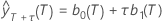 |
| b 0(T) | 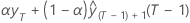 |
| b 1(T) |  |
MAPE
Mean absolute percentage error (MAPE) measures the accuracy of fitted time series values. MAPE expresses accuracy as a percentage.
Formula
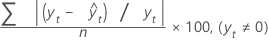
Notation
| Term | Description |
|---|---|
| yt | actual value at time t |
 | fitted value |
| n | number of observations |
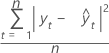
MAD
Mean absolute deviation (MAD) measures the accuracy of fitted time series values. MAD expresses accuracy in the same units as the data, which helps conceptualize the amount of error.
Formula
Notation
| Term | Description |
|---|---|
| yt | actual value at time t |
 | fitted value |
| n | number of observations |
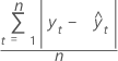
MSD
Mean squared deviation (MSD) is always computed using the same denominator, n, regardless of the model. MSD is a more sensitive measure of an unusually large forecast error than MAD.
Formula
Notation
| Term | Description |
|---|---|
| yt | actual value at time t |
 | fitted value |
| n | number of observations |