Methods and formulas for Box-Cox Transformation for Time Series

Common λ values

The following table shows some commonly used λ values and their transformations.

λ	Transformation
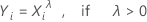
2
0.5
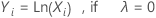
0
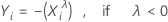
−1

Sub-series

Divide the series into sub-series by seasonal period. If the seasonal period does not divide evenly into the series, omit the remaining observations from the beginning of the series. If the specifications for the analysis do not include a seasonal period, then set the seasonal period = 2.

For example, assume an original time series with 10 observations and a seasonal period of 4: {5, 6, 3, 2, 9, 8, 1, 7, 10, 4}. The number of sub-series is 10 modulo 4 = 2. Because 4 does not divide evenly into 10, use only the last 8 observations to form the sub-series. The sub-series are {3, 2, 9, 8} and {1, 7, 10, 4}.

Missing values

If a sub-series contains 1 or more missing values, omit the sub-series from the calculations in the search for the optimal value of λ. The search requires at least 2 sub-series with no missing values.

Coefficient of variation

Term	Description
X1, X2, … XN	the observations in the original time series
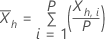
P	the seasonal period of the original time series
Xh, i	the ith observation in subseries h, where i=1, …, P and h=1, …, H
	the sample mean of the hth sub-series
	the sample standard deviation of the hth sub-series

The following equations define the statistics for each sub-series:

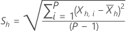
For a given λ and for h=1, …, H use the following definition:

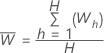
Calculate the sample average and the sample standard deviation for the W statistics:

The Coefficient of Variation (CV) for the W statistics has the following equation:

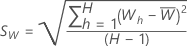
Use the method from Brent to find the value of λ that minimizes the CV in the interval from the specifications for the analysis. The analysis rounds the optimal value of λ to 0.5 or to the nearest integer to perform the transformation.