An analyst collected data on the number of airline passengers for 108 months. The analyst wants to use an ARIMA model to generate forecasts for the data. On a time series plot, the analyst sees that the difference between the high and low seasonal peaks grows over time. This pattern indicates that the variance is not stationary. The analyst performs a Box-Cox transformation to make the variance stationary before the analyst fits the ARIMA model.
- Open the sample data AirPassengers.MWX.
- Choose .
- In Series, enter Number of Passengers.
- In Seasonal period, enter 12.
- Select Optimal λ so that Minitab Statistical Software searches for a transformation to use.
- In Stamp column for time scale, enter Date.
- In Store transformed series in, enter Transformed. Click OK.
Interpret the results
The Method table shows the settings for the analysis and the value of λ for the transformation.
In these results, the seasonal period is 12 and the analysis searches for a λ value between the default range of -1 and 2. The optimal value for λ is approximately -0.14. The analysis rounds the value to 0 and uses the natural log transformation.
Method
| Seasonal period | 12 |
|---|---|
| Select optimal λ from interval | [-1, 2] |
| Optimal λ | -0.144439 |
| Rounded optimal λ | 0 |
| Transformed series = ln(Number of Passengers) |
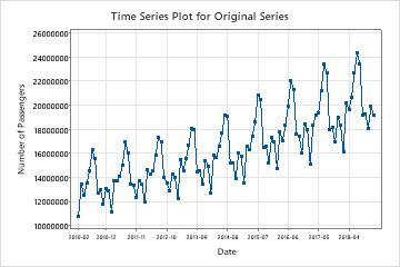
Compare the time series of the original series to the time series plot of the transformed series to verify that the transformation makes the variance stationary.
In these results, the time series plot of the original series shows the non-stationary variance. In this data, the difference between the high and low points in a seasonal cycle increases as time passes. This pattern shows that the variance increases as time passes.
Examine the time series plot of the transformed series to verify that the transformation makes the variance stationary.
In these results, the time series plot of the transformed series shows an approximately even difference between the high and low points in the seasonal cycles. This pattern shows that the transformation makes the variance stationary.
Also examine the time series plot of the transformed data to assess other important characteristics of the transformed series. For example, the assumptions for an ARIMA model include that the series has a stationary mean in addition to a stationary variance. If a time series plot of the transformed series shows that the transformed series does not have a stationary mean, try Augmented Dickey-Fuller Test to see whether differencing the data makes the mean of the series stationary.
In these results, the transformed series shows an upwards trend. This pattern shows that the mean of the series is not stationary. Use the Augmented Dickey-Fuller Test on the stored column of transformed data to determine if differencing makes the series stationary.