Regression models
| Term | Description |
|---|---|
 | the observed time series values at time = 1, …, T |
 | the difference of two consecutive observations at time
t,  ,
where
t = 2, …,
T ,
where
t = 2, …,
T |
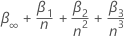
 | the constant term in a regression model |
 | the coefficient of a linear time trend in a regression model |
 | the coefficient of a quadratic time trend in a regression model |
 | the lag order of the autoregressive process |
 | the serially independent error term at time t for t = 2, ..., T |
- A model with only a constant coefficient

- A model with a constant coefficient and a linear coefficient

- A model with a constant coefficient, linear coefficient, and a quadratic coefficient

- A model with no regression coefficients

Hypotheses
Each Augmented Dickey-Fuller test uses the following hypotheses:
Null hypothesis, H0: 
Alternative hypothesis, H1: 
The null hypothesis says that a unit root is in the time series sample, which means that the mean of the data is not stationary. Rejecting the null hypothesis indicates that the mean of the data is stationary or trend stationary, depending on the model for the test.
Test statistic

where
| Term | Description |
|---|---|
 | the least square coefficient estimate of the
 coefficient
 |
 | the standard error of the least squares estimate of the
 coefficient from the regression model
 |
MacKinnon's approximate p-values
Under the null hypothesis, the asymptotic distribution of the test statistic does not follow a standard distribution. Fuller (1976)1 provides a table with common percentiles of the asymptotic distribution. MacKinnon (19942, 20103) applies response surface approximations to simulated data to provide an approximate p-value for any value of the ADF test statistic.
If the specifications for the analysis use 0.01, 0.05, or 0.1 as the significance level, then the evaluation of the null hypothesis compares the test statistic to the critical value for that significance level. If the test statistic is less than or equal to the critical value, reject the null hypothesis.
If the specifications for the analysis give a different significance level, then the evaluation of the null hypothesis compares the approximate p-value to the significance level. If the p-value is less than the significance level, reject the null hypothesis.
Critical values for the significance levels 0.01, 0.05, and 0.1
where
n is the number of observations that the analysis uses to fit the
regression model. The values for  and
and  come from tables in MacKinnon (2010). If the test statistic is less than or
equal to the critical value, reject the null hypothesis.
come from tables in MacKinnon (2010). If the test statistic is less than or
equal to the critical value, reject the null hypothesis.
Approximate p-values
The calculation of the approximate p-value comes from Mackinnon (1994). Compare the p-value to the significance level to make a decision. If the p-value is less than or equal to the significance level, reject the null hypothesis.
Determination of lag order

The selection of the lag order depends on the criterion in the specifications of the analysis. If the specifications for the analysis do not include a criterion, then the regression model for the test is the maximum order of p.
In the calculations to determine the lag order, the number of observations depends on the maximum lag order such that m = n – p – 1.
| Term | Description |
|---|---|
| n | the total number of observations |
| p | the maximum lag order of the differenced terms that are in the model |
The calculation of each criteria follows:
Akaike Information Criterion (AIC)
The analysis evaluates a regression model for each lag order in the specifications of the analysis. The lag order for the test is the regression model with the minimum value of the AIC.

where
| Term | Description |
|---|---|
| m | the number of observations that depends on the maximum lag order |
| k | the number of coefficients in the model, including the constant if the regression model has a non-zero constant |
| RSS | the residual sum of squares of the regression model |
Bayesian Information Criterion (BIC)
The analysis evaluates a regression model for each lag order in the specifications of the analysis. The lag order for the test is the regression model with the minimum value of the BIC.

where
| Term | Description |
|---|---|
| m | the number of observations that depends on the maximum lag order |
| k | the number of coefficients in the model, including the constant if the regression model has a non-zero constant |
| RSS | the residual sum of squares of the regression model |
t-statistic
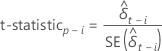
where i = 1, …, p
| Term | Description |
|---|---|
 | the least squares estimate of the  coefficient in the regression model
 |
 | the standard error of the least squares estimate of the
 coefficient in the regression model
 |