In This Topic
Coefficients
The coefficients are estimated using an iterative algorithm that calculates least squares estimates. At each iteration, the back forecasts are computed and SSE is calculated. For more details, see Box and Jenkins1.
The ARIMA algorithm is based on the fitting routine in the TSERIES package written by Professor William Q. Meeker, Jr., of Iowa State University2. We are grateful to Professor Meeker for his help in the adaptation of his routine to Minitab.
Back forecasts
Back forecasts are calculated using the specified model and the current iteration's parameter estimates. For more details, see Cryer3.
SSE
Formula

Notation
| Term | Description |
|---|---|
| n | total number of observations |
 | residuals using that iteration's parameter estimates, including back forecasts |
SS for residuals
Formula

Notation
| Term | Description |
|---|---|
| n | total number of observations |
| at | residuals using the final parameter estimates, excluding back forecasts |
DF for residuals
Formula
For a nonseasonal model with a constant term:
(n – d) – p – q – 1
For a nonseasonal model without a constant term:
(n – d) – p – q
For a seasonal model with a constant term:
(n – d −D×s) – p – q − P − Q – 1
For a seasonal model without a constant term
(n – d −D×s) – p – q − P − Q
Notation
| Term | Description |
|---|---|
| n | total number of observations |
| d | number of nonseasonal differences |
| p | number of nonseasonal autoregressive parameters included in the model |
| q | number of nonseasonal moving average parameters included in the model |
| D | number of seasonal differences |
| s | length of the seasonal period |
| P | number of seasonal autoregressive parameters included in the model |
| Q | number of seasonal moving average parameters included in the model |
MS for residuals
Formula
SS / DF
Chi-square statistic
Formula
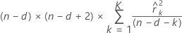
Notation
| Term | Description |
|---|---|
| n | total number of observations |
| d | number of differences |
| K | 12, 24, 36, 48 |
| k | lag |
 | autocorrelation of the residuals for the k th lag |
DF for chi-square statistic
Formula
For a nonseasonal model with a constant term:
K – p – q – 1
For a nonseasonal model without a constant term:
K – p – q
For a seasonal model with a constant term:
K – p – q − P − Q – 1
For a seasonal model without a constant term
K – p – q− P − Q
Notation
| Term | Description |
|---|---|
| K | 12, 24, 36, 48 |
| p | number of nonseasonal autoregressive parameters included in the model |
| q | number of nonseasonal moving average parameters included in the model |
| P | number of seasonal autoregressive parameters included in the model |
| Q | number of seasonal moving average parameters included in the model |
P-value for chi-square statistic
Formula
P(X < χ 2)
Notation
| Term | Description |
|---|---|
| X | distributed as χ 2 (DF) |
Forecasts
Formula
Forecasts are calculated recursively, based on the model and the parameter estimates. For more details, see Box and Jenkins1. For example, if an ARIMA model is fit with 1 autoregressive term (AR(1)) and one seasonal differencing term with a seasonal period of 12, this model is fit:
Yt – Yt–12 = γ + Φ(Yt–1 – Yt–12–1)
To estimate  , the first forecast, where k is the origin, find:
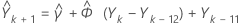
Then, you find  , in the same manner, and so on.
To calculate the 95% prediction interval for the forecast, first you have to calculate the weights.
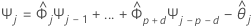
where  ,
,  for j < 0, and
  for j > q.
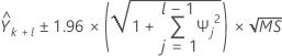
Notation
| Term | Description |
|---|---|
| Yt | actual value at time t |
| Φ | autoregressive term |
 | estimated autoregressive term |
| γ | constant term |
| d | number of differences |
| p | number of autoregressive parameters |
| q | number of moving average parameters |
 | estimated moving average term |
 | estimated constant term |
| MS | mean square error |