In This Topic
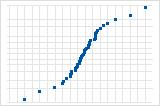
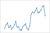
Time Series Plot
The time series plot displays the data in chronological order. When you generate forecasts, Minitab displays the forecasts and their 95% confidence limits on the plot.
Interpretation
- Determine whether different variations are present in the data. If different variations are present, then you must transform the data so that the variance is constant.
- Determine whether the data are centered around a constant mean. If the mean is not constant, you may need to difference the data to make the mean constant.
ACF of Residuals
The plot shows the autocorrelation function of the residuals. The autocorrelation function is a measure of the correlation between the observations of a time series that are separated by k time units (yt and yt–k).
Interpretation
Use the autocorrelation function of the residuals to determine whether the model meets the assumptions that the residuals are independent. If the assumption is not met, the model may not fit the data and you should use caution when you interpret the results. If no significant correlations are present, then you can conclude that the residuals are independent. However, you may see 1 or 2 significant correlations at higher order lags that are not seasonal lags. These lags are usually due to random error, and are not a sign that the assumption is not met. So, in this case, you can also conclude that the residuals are independent.
PACF of Residuals
The partial autocorrelation function is a measure of the correlation between the observations of a time series that are separated by k time units (yt and yt–k), after adjusting for the presence of all the other terms of shorter lag (yt–1, yt–2, ..., yt–k–1).
Interpretation
Use the partial autocorrelation function of the residuals to determine whether the model meets the assumptions that the residuals are independent. If the assumption is not met, the model may not fit the data and you should use caution when you interpret the results. If no significant correlations are present, then you can conclude that the residuals are independent.
Histogram of the residuals
The histogram of the residuals shows the distribution of the residuals for all observations. lf the model fits the data well, the residuals should be random with a mean of 0. So the histogram should be approximately symmetric around 0.
Normal probability plot of the residuals
The normal plot of the residuals displays the residuals versus their expected values when the distribution is normal.
Interpretation
Use the normal plot of the residuals to determine whether the residuals are normally distributed. However, this analysis does not require normally distributed residuals.
S-curve implies a distribution with long tails.

Inverted S-curve implies a distribution with short tails.
Downward curve implies a right-skewed distribution.
A few points lying away from the line implies a distribution with outliers.
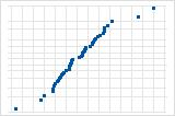
Residuals versus fits
The residuals versus fits plot displays the residuals on the y-axis and the fitted values on the x-axis.
Interpretation
Use the residuals versus fits plot to determine whether the residuals are unbiased and have a constant variance. Ideally, the points should fall randomly on both sides of 0, with no recognizable patterns in the points.
| Pattern | What the pattern may indicate |
|---|---|
| Fanning or uneven spreading of residuals across fitted values | Nonconstant variance |
| Curvilinear | A missing higher-order term |
| A point that is far away from zero | An outlier |
If you see nonconstant variance or patterns in the residuals, your forecasts may not be accurate.
Residuals versus order
The residuals versus order plot displays the residuals in the order that the data were collected.
Interpretation
Use the residuals versus order plot to determine how accurate the fits are compared to the observed values during the observation period. Patterns in the points may indicate that model does not fit the data. Ideally, the residuals on the plot should fall randomly around the center line.
| Pattern | What the pattern may indicate |
|---|---|
| A consistent long-term trend | The model does not fit the data |
| A short-term trend | A shift or a change in pattern |
| A point that is far away from the other points | An outlier |
| A sudden shift in the points | The underlying pattern for the data has changed |
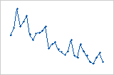
Residuals systematically decrease as the order of the observations increases from left to right.
A sudden change in the values of the residuals occurs from low (left) to high (right).
Residuals versus variables
The residuals versus variables plot displays the residuals versus another variable.
Interpretation
Use the plot to determine whether the variable affects the response in a systematic way. If patterns are present in the residuals, the other variables are associated with the response. You can use this information as the basis for additional studies.