Engineers want to assess the reliability of a redesigned compressor case of jet engines. To test the design, the engineers use a machine to throw a single projectile into each compressor case. After the projectile impact, engineers inspect the compressor every twelve hours for failure.
The engineers perform regression with life data to evaluate the relationship between the case design, the projectile weight, and the failure time. They also want to estimate the failure times at which they can expect 1% and 5% of the engines to fail. The engineers use a Weibull distribution to model the data.
- Open the sample data, JetEngineReliability.MWX.
- Choose .
- Select Responses are uncens/arbitrarily censored data.
- In Variables/Start variables, enter Start.
- In End variables, enter End.
- In Model, enter Design and Weight.
- In Factors (optional), enter Design.
- Click Estimate. In Enter new predictor values, enter New Design New Weight.
- In Estimate percentiles for percents, enter 1 5, then click OK.
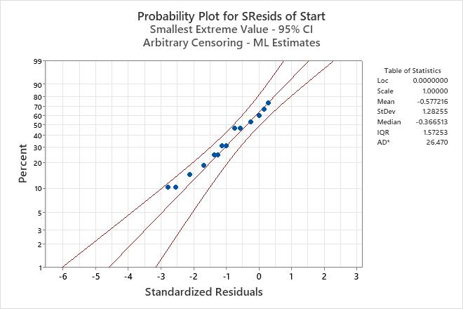
- Click Graphs. Select Probability plot for standardized residuals.
- Click OK in each dialog box.
Interpret the results
In the regression table, the p-values for design and weight are significant at an α-level of 0.05. Therefore, the engineers conclude that both the case design and the projectile weight have a statistically significant effect on the failure times. The coefficients for the predictors can be used to define an equation that describes the relationship between the case design, the projectile weight, and the failure time for the engines.
The table of percentiles shows the 1st and 5th percentiles for each combination of case design and projectile weight. The time that passes before 1% or 5% of the engines fail is longer for the new case design than the standard case design, at all the projectile weights. For example, after being subject to a 10-pound projectile, 1% of the engines with a standard case design can be expected to fail after approximately 101.663 hours. With the new case design, 1% of the engines can be expected to fail after approximately 205.882 hours.
The probability plot of the standardized residuals shows that the points follow an approximate straight line. Therefore, the engineers can assume that the model is appropriate.
Censoring
| Censoring Information | Count |
|---|---|
| Right censored value | 25 |
| Interval censored value | 23 |
Regression Table
| Standard Error | 95.0% Normal CI | |||||
|---|---|---|---|---|---|---|
| Predictor | Coef | Z | P | Lower | Upper | |
| Intercept | 6.68731 | 0.193766 | 34.51 | 0.000 | 6.30754 | 7.06709 |
| Design | ||||||
| Standard | -0.705643 | 0.0725597 | -9.72 | 0.000 | -0.847857 | -0.563428 |
| Weight | -0.0565899 | 0.0212396 | -2.66 | 0.008 | -0.0982187 | -0.0149611 |
| Shape | 5.79286 | 1.07980 | 4.02001 | 8.34755 | ||
Anderson-Darling (adjusted) Goodness-of-Fit
Table of Percentiles
| Standard Error | 95.0% Normal CI | |||||
|---|---|---|---|---|---|---|
| Percent | Design | Weight | Percentile | Lower | Upper | |
| 1 | Standard | 5.0 | 134.911 | 17.6574 | 104.385 | 174.363 |
| 1 | Standard | 7.5 | 117.113 | 16.0279 | 89.5591 | 153.144 |
| 1 | Standard | 10.0 | 101.663 | 16.3830 | 74.1295 | 139.423 |
| 1 | New | 5.0 | 273.214 | 36.8022 | 209.819 | 355.763 |
| 1 | New | 7.5 | 237.171 | 32.6878 | 181.028 | 310.726 |
| 1 | New | 10.0 | 205.882 | 32.8675 | 150.568 | 281.518 |
| 5 | Standard | 5.0 | 178.749 | 16.9676 | 148.404 | 215.300 |
| 5 | Standard | 7.5 | 155.168 | 14.1107 | 129.836 | 185.443 |
| 5 | Standard | 10.0 | 134.698 | 15.4568 | 107.568 | 168.670 |
| 5 | New | 5.0 | 361.994 | 36.0778 | 297.761 | 440.084 |
| 5 | New | 7.5 | 314.239 | 28.8741 | 262.450 | 376.247 |
| 5 | New | 10.0 | 272.783 | 30.6102 | 218.928 | 339.887 |