In This Topic
Probability plot
- Plot points, which are the estimated percentiles for corresponding probabilities of an ordered data set.
- Fitted line, which is the expected percentile from the distribution based on maximum likelihood parameter estimates.
- Confidence intervals, which are the confidence intervals for the percentiles.
Because the plot points do not depend on any distribution, they would be the same (before being transformed) for any probability plot made. However, the fitted line differs depending on the parametric distribution chosen. So you can use the probability plot to assess whether a particular distribution fits your data. In general, the closer the points fall to the fitted line, the better the fit.
Plot points
- Median rank method (default)
- Modified Kaplan-Meier method
- Herd-Johnson method
- Kaplan-Meier method
If the data contain tied failure times (identical failure times), either all points (default), the average (median), or the maximum of the tied points is plotted. If the tie involves failures and suspensions, the failures are considered to occur before the suspensions.
Each of these methods generates nonparametric estimates of F(t), the cumulative distribution function for the random variable T, which is time to failure.
For a sample of n observations, let x(1), x(2),...,x(n) be the order statistics, or the data ordered from smallest to largest. Then i is the rank of the I th ordered observation x(I). The formula for each method is as follows:
Median rank (Benard's method)
Formula for uncensored data

Formula for censored data

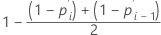
Modified Kaplan-Meier
Formula for uncensored data

Formula for censored data
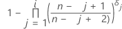
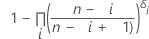
Herd-Johnson estimate
Formula for uncensored data

Formula for censored data
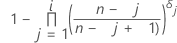
Kaplan-Meier product limit estimate
Note
If the largest observation is uncensored, the Kaplan-Meier method results in p = 1 for the largest uncensored observation. In this case, the Kaplan-Meier estimate for the largest observation results in a number that cannot be used in the plot. This problem is corrected by recalculating the largest p as 90% of the distance between the prior p and 1.
Note
For arbitrarily-censored data, Minitab estimates the cumulative probabilities using the Turnbull method1.
Formula for uncensored data

Formula for censored data
Notation
| Term | Description |
|---|---|
| i | rank of the data point, with ties given consecutive ranks |
| n | number of observations in the data |
| δj | 0 if the j th observation is censored, or 1 if the j th observation is uncensored |
| ARi |
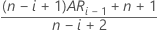 |
| AR0 | equals 0 |
| p'i |
 |
Fitted line
- Minitab transforms the x-axis to a log scale when you are using the Weibull, 3-parameter Weibull, exponential, lognormal, or loglogistic distribution.
- Minitab transforms the y-axis to a percent scale by default. If you change the y-scale type to probability, Minitab transforms the y-axis to a probability scale.
| Distribution | x coordinate | y coordinate |
|---|---|---|
| Smallest extreme value | failure time | ln(–ln(1 – p)) |
| Weibull | ln(failure time) | ln(–ln(1 – p)) |
| 3-parameter Weibull | ln(failure time – threshold) | ln(–ln(1 – p)) |
| Exponential | ln(failure time) | ln(–ln(1 – p)) |
| 2-parameter exponential | ln(failure time – threshold) | ln(–ln(1 – p)) |
| Normal | failure time | Φ –1 (p) |
| Lognormal | ln(failure time) | Φ –1 (p) |
| 3-parameter lognormal | ln(failure time – threshold) | Φ –1 (p) |
| Logistic | failure time |
 |
| Loglogistic | ln(failure time) |
 |
| 3-parameter loglogistic | ln(failure time – threshold) |
 |
Notation
| Term | Description |
|---|---|
| Φ –1 | inverse cdf for the standard normal distribution |
| ln (x) | natural log of x |