A reliability engineer studies the failure rates of engine windings of turbine assemblies to determine the times at which the windings fail. At high temperatures, the windings might decompose too fast.
The engineer records failure times for the engine windings at various temperatures. However, some of the units must be removed from the test before they fail. Therefore, the data are right censored. To select a distribution model for the data collected at 80° C, the engineer uses Distribution ID Plot (Right Censoring.
- Open the sample data, EngineWindingReliability.MWX.
- Choose .
- In Variables, enter Temp80.
- Select Specify. Ensure that the default distributions are selected (Weibull, Lognormal, Exponential, and Normal).
- Click Censor. Under Use censoring columns, enter Cens80.
- In Censoring value, type 0.
- Click OK in each dialog box.
Interpret the results
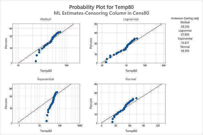
The points for the failure times fall approximately on the straight line on the lognormal probability plot. Therefore, the lognormal distribution provides a good fit. The engineer thus decides to use the lognormal distribution to model the data collected at 80° C.
Minitab also displays a table of percentiles and a table of mean time to failure (MTTF), which provide calculated failure times for each distribution. You can compare the calculated values to see how your conclusions may change with different distributions. If several distributions fit your data well, you may want to use the distribution that provides the most conservative results.
Goodness-of-Fit
| Distribution | Anderson-Darling (adj) |
|---|---|
| Weibull | 68.204 |
| Lognormal | 67.800 |
| Exponential | 70.871 |
| Normal | 68.305 |
Table of Percentiles
| Standard Error | 95% Normal CI | ||||
|---|---|---|---|---|---|
| Distribution | Percent | Percentile | Lower | Upper | |
| Weibull | 1 | 10.0765 | 2.78453 | 5.86263 | 17.3193 |
| Lognormal | 1 | 19.3281 | 2.83750 | 14.4953 | 25.7722 |
| Exponential | 1 | 0.809731 | 0.133119 | 0.586684 | 1.11758 |
| Normal | 1 | -0.549323 | 8.37183 | -16.9578 | 15.8592 |
| Weibull | 5 | 20.3592 | 3.79130 | 14.1335 | 29.3273 |
| Lognormal | 5 | 26.9212 | 3.02621 | 21.5978 | 33.5566 |
| Exponential | 5 | 4.13258 | 0.679391 | 2.99422 | 5.70371 |
| Normal | 5 | 18.2289 | 6.40367 | 5.67790 | 30.7798 |
| Weibull | 10 | 27.7750 | 4.11994 | 20.7680 | 37.1463 |
| Lognormal | 10 | 32.1225 | 3.09409 | 26.5962 | 38.7970 |
| Exponential | 10 | 8.48864 | 1.39552 | 6.15037 | 11.7159 |
| Normal | 10 | 28.2394 | 5.48103 | 17.4968 | 38.9820 |
| Weibull | 50 | 62.6158 | 4.62515 | 54.1763 | 72.3700 |
| Lognormal | 50 | 59.8995 | 4.31085 | 52.0192 | 68.9735 |
| Exponential | 50 | 55.8452 | 9.18089 | 40.4622 | 77.0766 |
| Normal | 50 | 63.5518 | 4.06944 | 55.5759 | 71.5278 |
Table of MTTF
| Standard Error | 95% Normal CI | |||
|---|---|---|---|---|
| Distribution | Mean | Lower | Upper | |
| Weibull | 64.9829 | 4.6102 | 56.5472 | 74.677 |
| Lognormal | 67.4153 | 5.5525 | 57.3656 | 79.225 |
| Exponential | 80.5676 | 13.2452 | 58.3746 | 111.198 |
| Normal | 63.5518 | 4.0694 | 55.5759 | 71.528 |