Interpret the key results for MARS^® Regression

Complete the following steps to interpret MARS^® Regression. Key output includes the model summary statistics, variable importance, the partial dependence plots, and the regression equation.

In This Topic

Step 1: Determine how well the model fits your data
Step 2: Determine which variables are most important to the model
Step 3: Explore the effects of the predictors

Step 1: Determine how well the model fits your data

To determine how well the model fits your data, examine the statistics in the Model Summary table. Usually, you use the test version of the statistics because the test version is a better representation of how the model performs for new data. If you fit additional models, use the values in the Model Summary table to compare how well the models fit the data.

Test R-squared: The higher the R² value, the better the model fits your data. R² is always between 0% and 100%. Outliers have a greater effect on R² than on MAD.
Test root mean squared error (RMSE): Smaller values indicate a better fit. Outliers have a greater effect on RMSE than on MAD.
Test mean squared error (MSE): Smaller values indicate a better fit. Outliers have a greater effect on MSE than on MAD.
Test mean absolute deviation (MAD): Smaller values indicate a better fit. The mean absolute deviation (MAD) expresses accuracy in the same units as the data, which helps conceptualize the amount of error. Outliers have less of an effect on MAD than on R², RMSE, and MSE.

Model Summary

Total predictors	77
Important predictors	10
Maximum number of basis functions	30
Optimal number of basis functions	13

Statistics	Training	Test
R-squared	89.61%	87.61%
Root mean squared error (RMSE)	25836.5197	27855.6550
Mean squared error (MSE)	667525749.7185	775937512.8264
Mean absolute deviation (MAD)	17506.0038	17783.5549

Key Results: Test R-squared, Test root mean squared error (RMSE), Test mean squared error (MSE), Test mean absolute deviation (MAD)

In these results, the test R-squared is about 88%. The test root mean squared error is about 27,856. The test mean squared error is about 775,937,513. The test mean absolute deviation is about 17,784.

Step 2: Determine which variables are most important to the model

Use the relative variable importance chart to see which predictors are the most important variables to the model.

Important variables are in at least 1 basis function in the model. The variable with the highest improvement score is set as the most important variable and the other variables are ranked accordingly. Relative variable importance standardizes the importance values for ease of interpretation. Relative importance is defined as the percent improvement with respect to the most important predictor.

Relative variable importance values range from 0% to 100%. The most important variable always has a relative importance of 100%. If a variable is not in a basis function, that variable is not important.

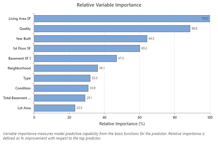
Key Result: Relative Variable Importance

In this example, the most important predictor variable is Living Area SF. If the contribution of the top predictor variable, Living Area SF, is 100%, then you can compare the other variables to Living Area SF to determine their importance. Thus, you can focus on the most important predictors. The following list describes the next most important variables in this model.

Quality is about 89% as important as Living Area SF.

Year Built is about 64% as important as Living Area SF.

1st Floor SF is about 60% as important as Living Area SF.

Although these results include 10 variables with positive importance, the relative rankings provide information about how many variables to control or monitor for a certain application. Steep drops in the relative importance values from one variable to the next variable can guide decisions about which variables to control or monitor. For example, in these data, the 2 most important variables have importance values that are relatively close together before a drop of over 20% in relative importance to the next variable. Similarly, 2 variables have similar importance values over 60%. You can remove variables from different groups and redo the analysis to evaluate how variables in various groups affect the prediction accuracy values in the model summary table.

Step 3: Explore the effects of the predictors

Use the partial dependence plots, the basis functions, and the coefficients in the regression equation to determine the effect of the predictors. The effects of the predictors explain the relationship between the predictors and the response. Consider all the basis functions for a predictor to understand the effect of the predictor on the response variable.

In addition, consider the use of the important predictors and the forms of their relationships when you build other models. For example, if the MARS^® regression model includes interactions, consider whether to include those interactions in a least-squares regression model to compare the performance of the two types of models. In applications where you control the predictors, the effects provide a natural way to optimize the settings to achieve a goal for the response variable.

In an additive model, one-predictor, partial dependence plots show how the important continuous predictors affect the predicted response. The one predictor partial dependence plot indicates how the response is expected to change with changes in the predictor levels. For MARS^® Regression, the values on the plot come from the basis functions for the predictor on the x-axis. The contribution on the y-axis is standardized so that the minimum value on the plot is 0.

Key Result: Partial dependence plot
This plot illustrates that Sale Price increases as the Living Area SF increases from the minimum square footage in the data set to about 3,000 square feet. After Living Area SF reaches 3,000 square feet, the contribution to Sale Price becomes flat at approximately $152,000.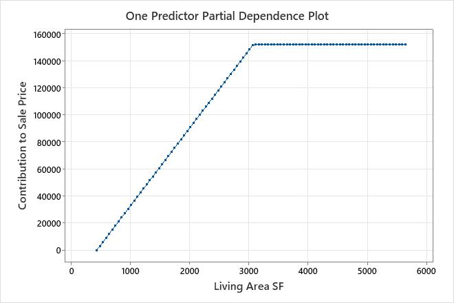

Regression Equation

BF2 = max(0, 3078 - Living Area SF)
BF3 = when Quality is 8, 9, 10
BF6 = max(0, 2002 - Year Built)
BF7 = when Basement SF 1 is not missing
BF10 = max(0, 1696 - Basement SF 1) * BF7
BF11 = when Quality is 1, 8
BF13 = when Type is 90, 150, 160, 180, 190
BF15 = when Neighborhood is Blueste, ClearCr, Crawfor, GrnHill, Landmrk, NoRidge, NridgHt,
     Somerst, StoneBr, Timber, Veenker
BF17 = when Total Basement SF is not missing
BF19 = max(0, Total Basement SF - 1392) * BF17
BF21 = max(0, 1st Floor SF - 2402)
BF23 = when Condition is 1, 2, 3, 4, 5, 6
BF25 = when Quality is 1, 7, 10
BF27 = max(0, 1st Floor SF - 2207)
BF30 = max(0, 15138 - Lot Area)

Sale Price = 325577 - 57.6167 * BF2 + 115438 * BF3 - 605.079 * BF6 - 25.3989 * BF10 -
     66735.2 * BF11 - 23688.9 * BF13 + 22374.5 * BF15 + 50.3801 * BF19 - 576.789 * BF21 - 18099.2
     * BF23 + 22414.2 * BF25 + 361.254 * BF27 - 1.82 * BF30

Key result: Regression equation

In these results, BF2 has a negative coefficient in the regression equation. The coefficient for the basis function is -57.6167. The arrangement of the basis function is max(0, c - X). In this arrangement, the value of the basis function decreases when the predictor increases. The combination of this arrangement and the negative coefficient creates a positive relationship between the predictor variable and the response variable. The slope of Living Area SF is 57.6167 from 438 to 3,078.

For more examples of common basis functions, go to Regression equation for MARS® Regression.

Interpret the key results for MARS® Regression