Row plot
Note
By default, Minitab displays the points for the first two principal components, which account for the greatest amount of total inertia. To display other principal components (axes) on the plot, click Graphs and enter the component numbers when you perform the analysis.
Interpretation
Use the row plot to look for relationships among row categories and to help interpret the principal components in relation to the row categories. Points that are farther away from the origin indicate categories that are more influential. Points on opposite sides of the plot indicate that a component contrasts these categories
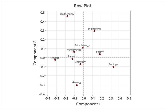
This row plot shows the row principal coordinates. Component 1, which best explains Zoology and Physics, shows these two fields farthest from the origin, but with opposite signs. Therefore, component 1 contrasts the biological sciences Zoology and Botany with Physics. Component 2 contrasts Biochemistry and Engineering with Geology.
Column plot
Note
By default, Minitab displays the points for the first two principal components, which account for the greatest amount of total inertia. To display other principal components (axes) on the plot, click Graphs and enter the component numbers when you perform the analysis.
Interpretation
Use the column plot to look for relationships among column categories and to help interpret the principal components in relation to the column categories. Points that are farther away from the origin indicate categories that are more influential. Points on opposite sides of the plot indicate that a component contrasts these categories.
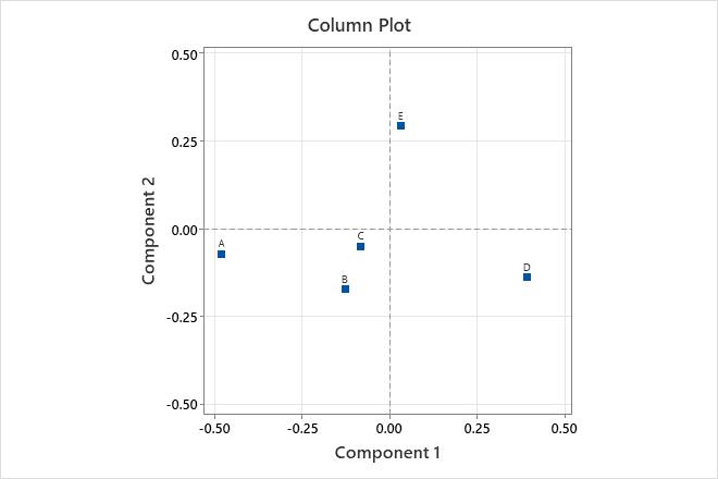
This column plot shows the column principal coordinates. Component 1, which best explains funding categories A and D, shows these two categories farthest from the origin, but with opposite signs. Therefore, component 1 contrasts these two funding categories. Component 2 best explains funding category E, and contrasts this category with the other funding categories.
Symmetric plot
Note
By default, Minitab displays the points for the first two principal components, which account for the greatest amount of total inertia. To display other principal components (axes) on the plot, click Graphs and enter the component numbers when you perform the analysis.
Interpretation
Important
The row-to-column distances in the symmetric plot use two different mappings. Because the row-to-column distances are not standardized, the distances between row categories and column categories cannot be interpreted easily. To interpret distances between row categories and column categories, use an asymmetric plot.
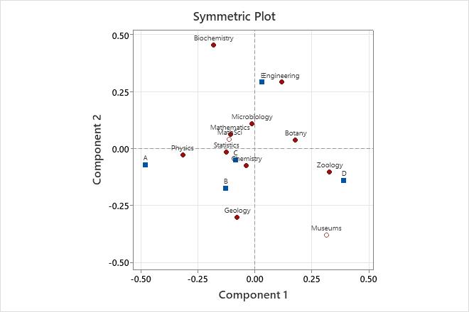
This symmetric plot shows the row and column principal coordinates. Component 1 best explains the row categories Zoology and Physics, and shows these two fields farthest from the origin, but with opposite signs. Component 1 contrasts the column category A with the column category D. Component 2 contrasts the row categories Biochemistry and Engineering with Geology and Museums, and best explains the column category E.
Asymmetric row plot
Note
By default, Minitab displays the points for the first two principal components, which account for the greatest amount of total inertia. To display other principal components (axes) on the plot, click Graphs and enter the component numbers when you perform the analysis.
Interpretation
Use the asymmetric row plot to look for relationships among the row and column categories and to help interpret the principal components. Points that are farther away from the origin indicate categories that are more influential. Points on opposite sides of the plot indicate that a component contrasts these categories. The closer a point for a row category is to a point for a column category, the higher the value of the row profile for the column category.
Note
Asymmetric plots allow you to intuitively interpret the distances between row points and column points, especially if the two components represent a large proportion of the total inertia. However, the points on an asymmetric plot might appear too close to each other in the center of the graph, which can make the results difficult to view. In that case, you may want to also display a symmetric plot to more clearly view the relationships among either the row or column categories.
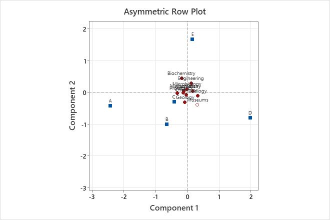
In this asymmetric row plot, the row points represent academic disciplines and the column points represent funding levels (A is the highest level of funding and D is the lowest. E indicates no funding).
Among funding classes, Component 1 contrasts levels of funding, while Component 2 contrasts being funded (A to D) with not being funded (E). Among the disciplines, Physics tends to have the highest funding level and Zoology has the lowest. Biochemistry tends to be unfunded, but when it is funded it is rarely in the lowest category of funding (D).Of the academic fields, Biochemistry is closest to column category E, implying that biochemistry as a discipline has the highest percentage of unfunded researchers in this study. Museums tend to be funded, but at a lower level than academic researchers. However, the cluster of points in the center of the graph make the results difficult to view. To more easily interpret the components in relation to the academic disciplines, also examine the asymmetric column plot or the symmetric row plot.
Asymmetric column plot
Note
By default, Minitab displays the points for the first two principal components, which account for the greatest amount of total inertia. To display other principal components (axes) on the plot, click Graphs and enter the component numbers when you perform the analysis.
Interpretation
Use the asymmetric column plot to look for relationships among the row and column categories and to help interpret the principal components. Points that are farther away from the origin indicate categories that are more influential. Points on opposite sides of the plot indicate that a component contrasts these categories. The closer a point for a column category is to a point for a row category, the higher the value of the column profile for the row category.
Note
Asymmetric plots allow you to intuitively interpret the distances between row points and column points, especially if the two components represent a large proportion of the total inertia. However, the points on an asymmetric plot might appear too close to each other in the center of the graph, which can make the results difficult to view. In that case, you may want to also display a symmetric plot to more clearly view the relationships among either the row or column categories.
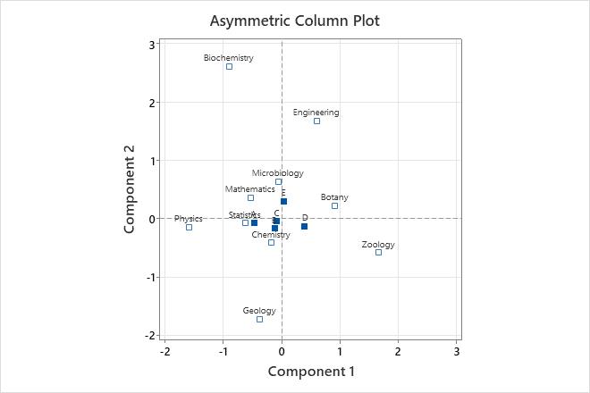
In this asymmetric column plot, the row points represent academic disciplines and the column points represent funding levels (A is the highest level of funding and D is the lowest. E indicates no funding).
Among disciplines, Component 1 contrasts Physics with Zoology, while Component 2 contrasts Biochemistry with Geology. Among funding classes, Component 1 contrasts levels of funding, while Component 2 contrasts being funded (A to D) with not being funded (E). Physics tends to have the highest funding level and Zoology has the lowest. Departments closer to the center of the plot tend to have funding profiles similar to the overall funding profile. Funding category E is closest to the row category Microbiology, which indicates that funding category E has the highest percentage of microbiology researchers.