Example of Simple Correspondence Analysis

A university research manager wants to determine how ten academic disciplines compare to each other in relation to five different funding categories. The manager collects 2-way classification data for 796 researchers.

For this two-way classification, the academic disciplines are rows and the funding categories are columns. A is the highest funding category, D is the lowest, and category E is unfunded. The manager performs a simple correspondence analysis to represent the associations between the rows and columns.

The manager also wants to examine supplementary data not included in the main data set. The supplementary data includes an additional row for museum researchers and a row for mathematical sciences, which is the sum of Mathematics and Statistics.

Open the sample data set, ResearchFunding.MTW.
Choose Stat > Multivariate > Simple Correspondence Analysis.
Under Input Data, select Columns of a contingency table and enter CT1-CT5. In Row names, enter RowNames. In Column names, enter ColNames.
Click Results and select Row profiles. Click OK.
Click Supp Data. In Supplementary Rows, enter RowSupp1 RowSupp2. In Row names, enter RSNames. Click OK.
Click Graphs. Select Show supplementary points in all plots. Select Symmetric plot showing rows only and Asymmetric row plot showing rows and columns.
Click OK in each dialog box.

Interpret the results

The Row Profiles table shows the proportions of each row category by column. For example, for Geology, 3.5% of the researchers are in funding category A, 22.4% are in funding category B, and so on. The mass for each row indicates the proportion of researchers in the entire data set. For example, the mass for Geology is 0.107, which indicates that 10.7% of the researchers are in the Geology field.

You can use the values in the Row Contributions and Column Contributions tables to interpret the different components. The column labeled Qual, or quality, indicates the proportion of the inertia represented by the two components.

For example, for the row contributions, the fields Zoology (0.929) and Geology (0.916) are best represented among the fields by the two component breakdown. Math has the poorest representation, with a quality value of 0.319. For the column contributions, the two components explain most of the variability in funding categories B, D, and E. The funded categories A, B, C, and D contribute most to component 1, while the unfunded category, E, contributes most to component 2.

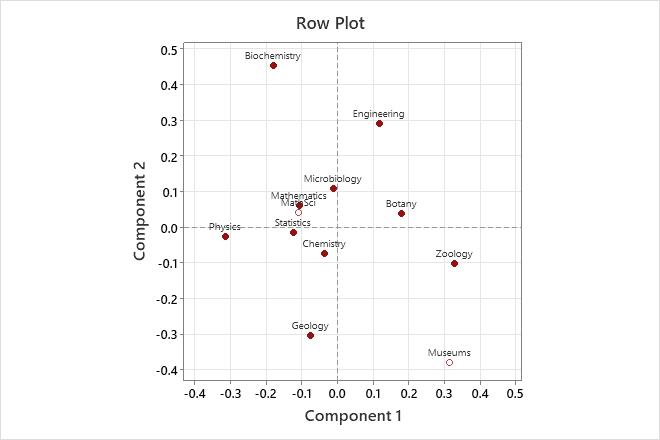
The row plot shows the row principal coordinates. Component 1, which best explains Zoology and Physics, shows these two fields farthest from the origin, but with opposite sign. Therefore, component 1 contrasts the biological sciences Zoology and Botany with Physics. Component 2 contrasts Biochemistry and Engineering with Geology.

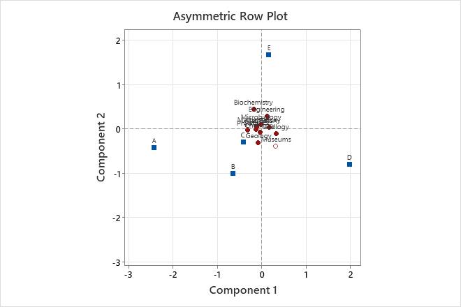
In the asymmetric row plot, the rows are scaled in principal coordinates and the columns are scaled in standard coordinates. Among funding classes, Component 1 contrasts levels of funding, while Component 2 contrasts being funded (A to D) with not being funded (E). Among the disciplines, Physics tends to have the highest funding level and Zoology has the lowest. Biochemistry tends to be in the middle of the funding level, but highest among unfunded researchers. Museums tend to be funded, but at a lower level than academic researchers.

	A	B	C	D	E	Mass
Geology	0.035	0.224	0.459	0.165	0.118	0.107
Biochemistry	0.034	0.069	0.448	0.034	0.414	0.036
Chemistry	0.046	0.192	0.377	0.162	0.223	0.163
Zoology	0.025	0.125	0.342	0.292	0.217	0.151
Physics	0.088	0.193	0.412	0.079	0.228	0.143
Engineering	0.034	0.125	0.284	0.170	0.386	0.111
Microbiology	0.027	0.162	0.378	0.135	0.297	0.046
Botany	0.000	0.140	0.395	0.198	0.267	0.108
Statistics	0.069	0.172	0.379	0.138	0.241	0.036
Mathematics	0.026	0.141	0.474	0.103	0.256	0.098
Mass	0.039	0.161	0.389	0.162	0.249

Axis	Inertia	Proportion	Cumulative
1	0.0391	0.4720	0.4720
2	0.0304	0.3666	0.8385
3	0.0109	0.1311	0.9697
4	0.0025	0.0303	1.0000
Total	0.0829

					Component 1			Component 2
ID	Name	Qual	Mass	Inert	Coord	Corr	Contr	Coord	Corr	Contr
1	Geology	0.916	0.107	0.137	-0.076	0.055	0.016	-0.303	0.861	0.322
2	Biochemistry	0.881	0.036	0.119	-0.180	0.119	0.030	0.455	0.762	0.248
3	Chemistry	0.644	0.163	0.021	-0.038	0.134	0.006	-0.073	0.510	0.029
4	Zoology	0.929	0.151	0.230	0.327	0.846	0.413	-0.102	0.083	0.052
5	Physics	0.886	0.143	0.196	-0.316	0.880	0.365	-0.027	0.006	0.003
6	Engineering	0.870	0.111	0.152	0.117	0.121	0.039	0.292	0.749	0.310
7	Microbiology	0.680	0.046	0.010	-0.013	0.009	0.000	0.110	0.671	0.018
8	Botany	0.654	0.108	0.067	0.179	0.625	0.088	0.039	0.029	0.005
9	Statistics	0.561	0.036	0.012	-0.125	0.554	0.014	-0.014	0.007	0.000
10	Mathematics	0.319	0.098	0.056	-0.107	0.240	0.029	0.061	0.079	0.012

					Component 1			Component 2
ID	Name	Qual	Mass	Inert	Coord	Corr	Contr	Coord	Corr	Contr
1	Museums	0.556	0.067	0.353	0.314	0.225	0.168	-0.381	0.331	0.318
2	MathSci	0.559	0.134	0.041	-0.112	0.493	0.043	0.041	0.066	0.007

					Component 1			Component 2
ID	Name	Qual	Mass	Inert	Coord	Corr	Contr	Coord	Corr	Contr
1	A	0.587	0.039	0.187	-0.478	0.574	0.228	-0.072	0.013	0.007
2	B	0.816	0.161	0.110	-0.127	0.286	0.067	-0.173	0.531	0.159
3	C	0.465	0.389	0.094	-0.083	0.341	0.068	-0.050	0.124	0.032
4	D	0.968	0.162	0.347	0.390	0.859	0.632	-0.139	0.109	0.103
5	E	0.990	0.249	0.262	0.032	0.012	0.006	0.292	0.978	0.699

Example of Simple Correspondence Analysis

Interpret the results

Row Profiles

Analysis of Contingency Table

Row Contributions

Supplementary Rows

Column Contributions