In This Topic
Column principal coordinate
Column profiles lie in a d-dimensional space. The full set of d principal axes span this space. Suppose gj1, gj2, gj3, ..., gjd are the coordinates of column profile j in terms of the principal axes. These coordinates are called the column principal coordinates. The kth principal coordinate for column profile j is gjk.
The best k-dimensional subspace is spanned by the first k principal axes. If we project column profile j onto the best k-dimensional subspace, gj1, ..., gjk are the column principal coordinates of the profile in this subspace.
Correlation
The correlation between column profile i and principal component k is calculated as follows:

Minitab calculates the relative inertia for each column. The absolute inertia is the product of the relative inertia and the total inertia.
The sum of the correlations for column j, over all principal components is 1. The sum over the first k principal coordinates is the quality associated with column profile j and the best k-dimensional subspace.
Notation
| Term | Description |
|---|---|
| gjk | kth principal coordinate for column profile j |
Inertia and cell inertia

The sum of all the cell inertias is the total inertia, sometimes simply called the inertia, for the table.

Principal axes (principal components)
Column profiles lie in a c-dimensional space. Lower dimensional subspaces are spanned by principal axes, also called principal components. The first principal axis is chosen as the vector in c-dimensional space that accounts for the maximum amount of the total inertia. Therefore, the first principal axis spans the best (that is, closest to the profiles using an appropriate metric) one-dimensional subspace. The second principal axis is chosen as the vector in c-dimensional space that accounts for the maximum amount of the remaining inertia. Therefore, the first two principal axes span the best two-dimensional subspace. The third principal axis is chosen as the vector in c-dimensional space that accounts for the maximum amount of the remaining inertia, after the inertia accounted for by the first two principal axes. Therefore, the first three principal axes span the best three-dimensional subspace, and so on.
Let d = the smaller of (r − 1) and (c − 1). The column profiles actually lie in a d dimensional subspace of the full c-dimensional space (or equivalently the full r-dimensional space). Thus, the number of principal axes is at most d.
Quality

Quality is always a number between 0 and 1, with larger numbers indicating a better approximation.
Notation
| Term | Description |
|---|---|
| gjk | kth principal coordinate for column profile j |
Relative contribution to total inertia

Column contributions

The sum of the contributions for principal axis k, over all columns j, is 1.
Notation
| Term | Description |
|---|---|
| gjk | kth principal coordinate for column profile j |
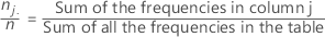
Column mass
The vector of c column masses is the same as the average column profile.
Standardized coordinates
The column standardized coordinates for component k are the principal coordinates for component k divided by the square root of the kth inertia.