In This Topic
Principal components
In the principal components extraction method, the jth loadings are the scaled coefficients of the jth principal components. The factors are related to the first m components. In the unrotated solution, you can interpret the factors as you would interpret the components in principal components analysis. However, after rotation, you can no longer interpret the factors similar to principal components.
The principal component factor analysis of the sample correlation matrix R (or covariance matrix S) is specified in terms of its eigenvalue-eigenvector pairs (λi, ei), i = 1, ...,p and λ1 ≤ λ2 ≤ ... ≤ λp. Let m < p be the number of common factors. The matrix of estimated factor loadings is a p × m matrix, L, whose ith column is  , i = 1, ..., m.
Maximum likelihood
The maximum likelihood method estimates the factor loadings, assuming the data follow a multivariate normal distribution. As its name implies, this method finds estimates of the factor loadings and unique variances by maximizing the likelihood function associated with the multivariate normal model. Equivalently, this is done by minimizing an expression involving the variances of the residuals. The algorithm iterates until a minimum is found or until the maximum specified number of iterations (the default is 25) is reached.
Minitab uses an algorithm based on Joreskog,1,2 with some adjustments to improve convergence. We give a brief summary of the algorithm here.
Suppose we have p variables and want to fit a model with m factors. Let R be the p × p correlation matrix of the variables, L be the p × m matrix of factor loadings, and Ψ be a p × p diagonal matrix whose diagonal elements are the unique variances, Ψi. Then we need to find values for L and Ψ that maximize the likelihood function, f(L,Ψ). This involves a two-step procedure, first finding a value for Ψ, then for L.
You can indirectly specify the initial value of Ψ. In the Factor Analysis - Options subdialog box, enter the column containing the initial values for the communalities in Use initial communality estimates in. Minitab then calculates the diagonal elements of Ψ as (1 − communalities).
For a fixed value of Ψ, we maximize f(L,Ψ) with respect to L. This is a simple matrix calculation. The value of L is then substituted into f(L,Ψ). Now f can be viewed as a function of Ψ. A simple transformation of this function gives

where λ1 < λ2 < ... λp are eigenvalues of Ψ R- 1Ψ. We then minimize g(Ψ), using a Newton-Raphson procedure. This gives an estimate of Ψ, which is then substituted into the likelihood f(L,Ψ). Then the likelihood is again maximized with respect to L. Then a new value for g(Ψ) is calculated, and so on. By default, iterations continue up to 25 steps if convergence is not achieved. If the algorithm does not convergence in 25 steps, you may want to change the default maximum number of iterations in the Options subdialog box.
Convergence is reached at step n, if either of the following are true:
- The function g(Ψ) does not change very much between consecutive steps. Specifically, if:
- | [g(Ψ) at step n] − [g(Ψ) at step (n − 1)] | < 10-6
- None of the unique variances change very much between consecutive steps. Specifically, if:
- | ln(Ψi at step n) − ln(Ψi at step n − 1) | < K2,
for all i = 1, ... , p, where Ψi the ith diagonal element of Ψ, is the unique variance corresponding to variable i.
The value of K2 can be specified in Convergence in the Options subdialog box. By default, the value is 0.005.
Choose All and MLE iterations in the Results subdialog box to display information on each iteration. The value of the objective function, g(Ψ), is displayed, then the maximum change in ln(Ψi). If, on an iteration, the value of g(Ψ) does not decrease, then a smaller (half the size) step is taken. Half-stepping is continued until g(Ψ) decreases or 25 half-steps are taken. The number of half steps is displayed. If g(Ψ) did not decrease in 25 half-steps, the algorithm stops and a message is displayed.
A matrix of second derivatives is used in the minimization of g(Ψ). This matrix is not always positive definite. If it is not, an approximation is used. An asterisk is displayed on the results when Minitab uses the exact matrix.
When minimizing the function g(Ψ), it is possible to find values of the diagonal element of Ψ that are 0 or negative. To prevent this, Minitab's algorithm bounds the diagonal elements of Ψ away from 0. Specifically, if a unique variance Ψi is less than K2, it is set equal to K2. K2 is the value set in Convergence in the Options subdialog box.
When the algorithm converges, a final check is performed on the unique variances. If any of the unique variances are less than K2, they are set equal to 0. The corresponding communality is then equal to 1. This result is called a Heywood case and Minitab displays a message to inform the user of this result. Optimization algorithms, such as the one used for maximum likelihood factor analysis, can give different answers with minor changes in the input. For example, if you change a few data points, change the starting values in Use initial communality estimates in, or change the convergence criterion in Convergence, you may see differences in factor analysis results. This is especially true if the solution lies in a relatively flat place on the maximum likelihood surface.
Rotating the loadings
An orthogonal rotation is an orthogonal transformation of the factor loadings that allows for easier interpretation of the factor loadings. The rotated loadings retain the correlation or covariance matrix, the residual matrix, the specific variances, and the communalities. Because the loadings change, the variance accounted by each factor and the corresponding proportion change.
Rotation places the axes close to as many points as possible and associates each group of variables with a factor. However, in some cases, a variable is close to more than one axis and is therefore associated with more than one factor.
You can choose from four rotation methods:
- Equimax - maximizes variance of squared loadings within both variables and factors.
- Varimax - maximizes variance of squared loadings within factors. This method simplifies the columns of the loading matrix and is the most widely used rotation method. To ease interpretation, this method attempts to make the loadings either large or small.
- Quartimax - maximizes variance of squared loadings within variables. This method simplifies the rows of the loading matrix.
- Orthomax with γ - rotation that comprises the above three depending on the value of the parameter gamma (0 - 1).
Factor analysis model
The factor analysis model is:
X = μ + L F + e
where X is the p x 1 vector of measurements, μ is the p x 1 vector of means, L is a p × m matrix of loadings, F is a m × 1 vector of common factors, and e is a p × 1 vector of residuals. Here, p represents the number of measurements on a subject or item and m represents the number of common factors. F and e are assumed to be independent and the individual F's are independent of each other. The mean of F and e are 0, Cov(F) = I, the identity matrix, and Cov(e) = Ψ, a diagonal matrix. The assumptions about independence of the F's make this an orthogonal factor model.
Under the factor analysis model, the p × p covariance matrix of the data, X, is calculated as follows:
Cov(X) = L L' + Ψ
where L is the p × m matrix of loadings, and Ψ is a p × p diagonal matrix. The ith diagonal element of L L', the sum of the squared loadings, is called the ith communality. The communality values can be judged as the percent of variability explained by the common factors. The ith diagonal element of Ψ is called the ith specific variance, or uniqueness. The specific variance is that portion of variability not explained by the common factors. The sizes of the communalities and/or the specific variances can be used to evaluate the goodness of fit.
Loadings
Formula
When the principal components method is used, the matrix of estimated factor loadings, L, is given by:
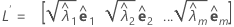
When the maximum likelihood method is used, the matrix of factor loadings is obtained through an iterative process.
Notation
| Term | Description |
|---|---|
 | eigenvalue-eigenvector pairs |
Communalities
Formula
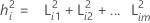
where i = 1, 2 ... p
Notation
| Term | Description |
|---|---|
| L | matrix of factor loadings |
Variance
Variability in the data explained by each factor. Variance equals the eigenvalue if you use principal components to extract factors and do not rotate the loadings.
% Var
Formula
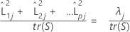
When a correlation matrix is used, the proportion of variance explained by the jth factor is calculated as follows:

Notation
| Term | Description |
|---|---|
| L | matrix of factor loadings |
| λj | jth eigenvalue |
| tr(R) | trace of correlation matrix |
| tr(S) | trace of covariance matrix |
Coefficients
Formula


R is the correlation matrix. If the matrix to factor is the covariance matrix, then R is replaced with the covariance matrix.
Notation
| Term | Description |
|---|---|
| L | matrix of the factor loadings |
Scores
Formula
F = ZC
Notation
| Term | Description |
|---|---|
| F | matrix of factor scores |
| Z | standardized data |
| C | matrix of factor score coefficients |