In This Topic
Step 1: Examine the similarity and distance levels
At each step in the amalgamation process, view the clusters formed and examine their similarity and distance levels. The higher the similarity level, the more similar (correlated) the variables are in each cluster. The lower the distance level, the closer the variables are in each cluster.
Ideally, the clusters should have a relatively high similarity level and a relatively low distance level. However, you must balance that goal with having a reasonable and practical number of clusters.
Amalgamation Steps
| Step | Number of clusters | Similarity level | Distance level | Clusters joined | New cluster | Number of obs. in new cluster | |
|---|---|---|---|---|---|---|---|
| 1 | 4 | 93.9666 | 0.120669 | 2 | 3 | 2 | 2 |
| 2 | 3 | 93.1548 | 0.136904 | 4 | 5 | 4 | 2 |
| 3 | 2 | 87.3150 | 0.253700 | 1 | 4 | 1 | 3 |
| 4 | 1 | 79.8113 | 0.403775 | 1 | 2 | 1 | 5 |
Key Results: Similarity level, Distance level
In these results, the data contain a total of 5 variables. In step 1, two clusters (variables 2 and 3 in the worksheet) are joined to form a new cluster. This creates 4 clusters in the data, with a similarity level of 93.9666 and a distance level of 0.130669. Although the similarity level is high and the distance level is low, the number of clusters is too high to be useful. At each subsequent step, as new clusters are formed, the similarity level decreases and the distance level increases. At the final step, all the variables are joined into a single cluster.
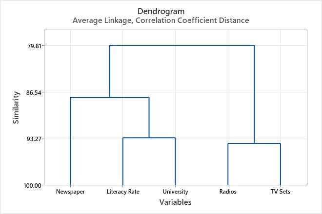
To view the similarity levels in the dendrogram, hold your pointer over a horizontal line in the tree diagram, in Minitab.
Step 2: Determine the final groupings for your data
Use the similarity level for the clusters that are joined at each step to help determine the final groupings for the data. Look for an abrupt change in the similarity level between steps. The step that precedes the abrupt change in similarity may provide a good cut-off point for the final partition. For the final partition, the clusters should have a reasonably high similarity level. You should also use your practical knowledge of the data to determine the final groupings that make the most sense for your application.
For example, the following amalgamation table shows that the similarity level decreases slightly from step 1 (93.9666) to step 2 (93.1548). The similarity then decreases abruptly in step 3 (87.3150), when the number of clusters changes from 3 to 2. These results indicate that 3 clusters may be appropriate for the final partition. If this grouping makes intuitive sense, then it is probably a good choice.
Amalgamation Steps
| Step | Number of clusters | Similarity level | Distance level | Clusters joined | New cluster | Number of obs. in new cluster | |
|---|---|---|---|---|---|---|---|
| 1 | 4 | 93.9666 | 0.120669 | 2 | 3 | 2 | 2 |
| 2 | 3 | 93.1548 | 0.136904 | 4 | 5 | 4 | 2 |
| 3 | 2 | 87.3150 | 0.253700 | 1 | 4 | 1 | 3 |
| 4 | 1 | 79.8113 | 0.403775 | 1 | 2 | 1 | 5 |
Key Results: Similarity level, Number of clusters
The decision about final grouping is also called cutting the dendrogram. Cutting the dendrogram is akin to drawing a horizontal line across the dendrogram to specify the final grouping. For example, to cut this dendrogram into four clusters, imagine drawing a horizontal line about halfway down the vertical axis, just below the similarity level of approximately 88.
Step 3: Examine the final partition
After you determine the final groupings in step 2, repeat the analysis and specify the number of clusters (or the similarity level) for the final partition. Minitab displays the final partition table, which shows the variables that form each cluster in the final partition.
Examine the clusters in the final partition to determine whether the grouping seems logical for your application. If you are still unsure, you can repeat the analysis, and compare dendrograms for different final groupings, to decide which one is the most logical for your data.
Amalgamation Steps
| Step | Number of clusters | Similarity level | Distance level | Clusters joined | New cluster | Number of obs. in new cluster | |
|---|---|---|---|---|---|---|---|
| 1 | 4 | 93.9666 | 0.120669 | 2 | 3 | 2 | 2 |
| 2 | 3 | 93.1548 | 0.136904 | 4 | 5 | 4 | 2 |
| 3 | 2 | 87.3150 | 0.253700 | 1 | 4 | 1 | 3 |
| 4 | 1 | 79.8113 | 0.403775 | 1 | 2 | 1 | 5 |
Final Partition
| Variables | |
|---|---|
| Cluster 1 | Newspaper |
| Cluster 2 | Radios TV Sets |
| Cluster 3 | Literacy Rate University |
Key Results: Final partition, dendrogram
In these results, the three clusters are formed in the final partition:
- Numbers of newspaper copies per 1,000 people
- Number of radios and television sets
- Literacy level and whether a university is located in the city
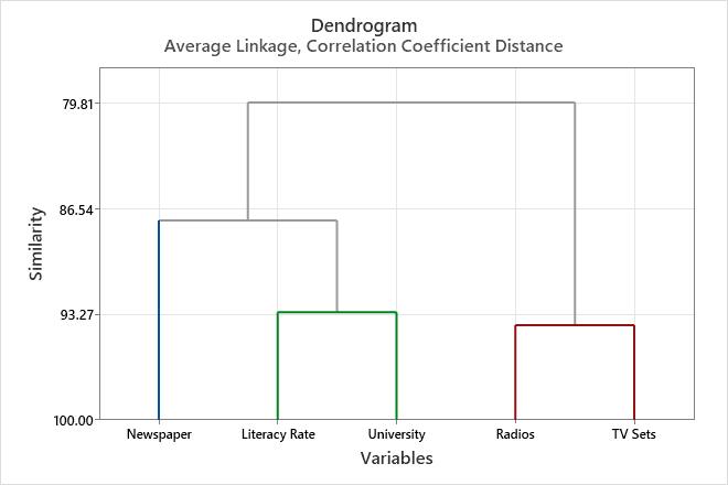
This dendrogram was created using a final partition of 3 clusters. Each final cluster is indicated by a separate color. The dendrogram was cut at a similarity level of approximately 88. If you cut the dendrogram higher, then there would be fewer final clusters, but the similarity level would be reduced. If you cut the dendrogram lower, then the similarity level would be greater, but there would be more final clusters.