Example of Individual Distribution Identification

Interpret the results

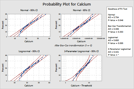
Minitab displays a probability plot and a p-value for each distribution and transformation. If a distribution is a good fit for the data (or if a transformation is effective), the points on the plot follow a straight line within the confidence bounds and the p-value is greater than the alpha level. An alpha level of 0.05 is often used. The p-value for the likelihood-ratio test (LRT) indicates whether adding an additional parameter to a distribution significantly improves its fit. An LRT p-value that is less than 0.05 suggests that the improvement is significant.

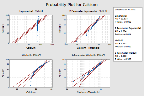
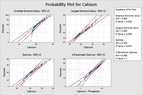
For these data, the 3-parameter Weibull distribution (p > 0.500) and the largest extreme value distribution (p > 0.250) are a good fit for the data. Adding a third parameter significantly improves the fit of the lognormal distribution (LRT P = 0.017), the Weibull distribution (LRT P = 0.000), the gamma distribution (LRT P = 0.006), and the loglogistic distribution (LRT P = 0.027).

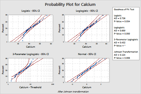
The Box-Cox transformation (p = 0.324) and the Johnson transformation (p = 0.986) are effective for these data. After the transformation, the normal distribution provides a good fit for the transformed values.

Descriptive Statistics

N	N*	Mean	StDev	Median	Minimum	Maximum	Skewness	Kurtosis
50	0	50.782	2.76477	50.4	46.8	58.1	0.644923	-0.287071

Box-Cox transformation: λ = -4

Johnson transformation function:

0.804604 + 0.893699 × Ln( ( X - 46.2931 ) / ( 59.8636 - X ) )

Goodness of Fit Test

Distribution	AD	P	LRT P
Normal	0.754	0.046
Box-Cox Transformation	0.414	0.324
Lognormal	0.650	0.085
3-Parameter Lognormal	0.341	*	0.017
Exponential	20.614	<0.003
2-Parameter Exponential	1.684	0.014	0.000
Weibull	1.442	<0.010
3-Parameter Weibull	0.230	>0.500	0.000
Smallest Extreme Value	1.656	<0.010
Largest Extreme Value	0.394	>0.250
Gamma	0.702	0.071
3-Parameter Gamma	0.268	*	0.006
Logistic	0.726	0.034
Loglogistic	0.659	0.050
3-Parameter Loglogistic	0.432	*	0.027
Johnson Transformation	0.124	0.986

ML Estimates of Distribution Parameters

Distribution	Location	Shape	Scale	Threshold
Normal*	50.78200		2.76477
Box-Cox Transformation*	0.00000		0.00000
Lognormal*	3.92612		0.05368
3-Parameter Lognormal	1.69295		0.46849	44.74011
Exponential			50.78200
2-Parameter Exponential			4.06326	46.71873
Weibull		17.82470	52.13681
3-Parameter Weibull		1.47605	4.53647	46.66579
Smallest Extreme Value	52.22257		2.95894
Largest Extreme Value	49.50370		2.16992
Gamma		351.04421	0.14466
3-Parameter Gamma		2.99218	1.63698	45.88376
Logistic	50.57182		1.59483
Loglogistic	3.92259		0.03121
3-Parameter Loglogistic	1.54860		0.32763	45.46180
Johnson Transformation*	0.02897		0.97293