In This Topic
Variance components
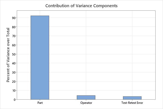
The Contribution of Variance Components plot and the Variance Components table show the variation from different sources.
Interpretation
Use the variance components to assess the variation from each source. The test-retest variance and the operator variance are measurement errors. The part variation represents the range of parts in the study. The total variance is the sum of the other components. If the analysis includes the interaction, then the amount of measurement error depends on which part an operator measures.
In an acceptable measurement system, the largest component of variation is part variation. If test-retest variation and operator variation contribute large amounts of variation, investigate the source of the problem and take corrective action.
Variance Components
| Source | Variance | %Total | StdDev |
|---|---|---|---|
| Test-Retest Error (Repeatability) | 0.03997 | 3.394 | 0.19993 |
| Operator (Reproducibility) | 0.05146 | 4.368 | 0.22684 |
| Part (Product variation) | 1.08645 | 92.238 | 1.04233 |
| Total | 1.17788 | 100.000 | 1.08530 |
Repeatability chart
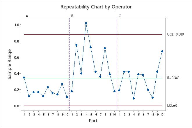
The repeatability chart is a control chart of ranges that displays operator consistency.
- Plotted points
- For each operator, the sample range is the difference between the largest and smallest measurements of each part. Use the sample ranges to evaluate operator consistency.
- Center line (Rbar)
- The grand average for the process (that is, average of all the sample ranges).
- Control limits (LCL and UCL)
- The amount of variation that you can expect for the sample ranges. To calculate the control limits, Minitab uses the variation within samples.
Note
If each operator measures each part 9 times or more, Minitab displays standard deviations on the chart instead of ranges.
Interpretation
The smaller the average range, the lower the variation from the measurement system. A point that is higher than the upper control limit (UCL) indicates that the operator does not measure parts consistently. The calculation of the UCL includes the number of measurements per part by each operator, and part variation. If the operators measure parts consistently, then the range between the highest and lowest measurements is small, relative to the study variation, and the points should be in control.
Signal-to-noise chart by operator
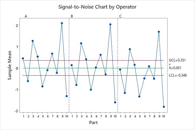
The chart compares the part variation to the test-retest component.
- Plotted points
- The average measurement of each part, plotted by each operator.
- Center line (
 )
) - The overall average for all part measurements by all operators.
- Control limits (LCL and UCL)
- The control limits are based on the repeatability estimate and the number of measurements in each average.
Interpretation
The parts that are chosen for a study should represent the entire range of possible parts. Thus, this graph should indicate more variation between part averages than what is expected from test-retest variation alone.
Ideally, the graph has narrow control limits with many out-of-control points that indicate a measurement system with low variation.
Parallelism plot
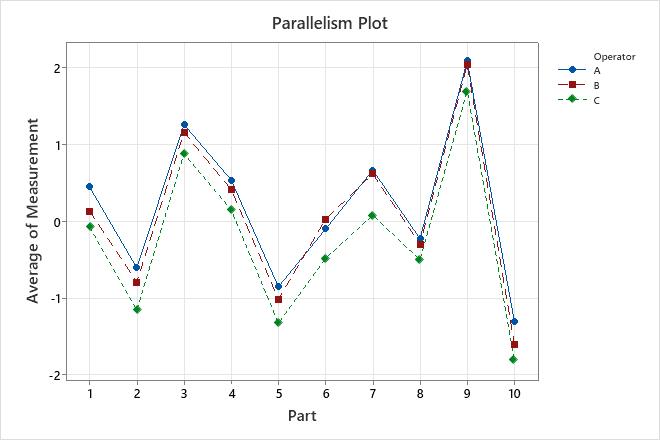
The parallelism plot displays the average measurements by each operator for each part. Each line connects the averages for a single operator.
The plot displays the interaction between two sources of variation: parts and operators. An interaction occurs when the effect of one factor is dependent on a second factor.
Interpretation
Lines that are coincident indicate that the operators measure similarly. Lines that are not parallel or that cross indicate that an operator's ability to measure a part consistently depends on which part is being measured. A line that is consistently higher or lower than the others indicates that an operator adds bias to the measurement by consistently measuring high or low.
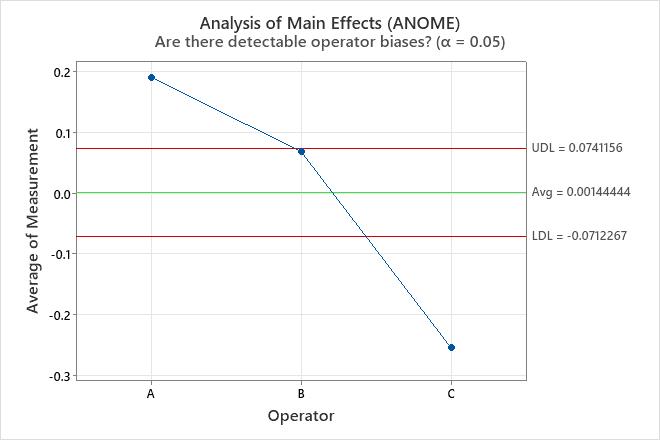
Analysis of main effects (ANOME) plot
The plot compares the average measurements for the operators.
- Plotted points
- The average measurement of all the parts for each operator.
- Center line (Avg)
- The overall average for all part measurements by all operators.
- Decision limits (LDL and UDL)
- The limits are based on the test-retest estimate and the number of measurements in each average.
Interpretation
Points outside of the decision limits indicate that different operators add bias to the measurements. Ideally, the points are all within the decision limits to indicate that the overall averages of the operators are similar.
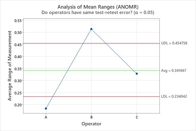
Analysis of mean ranges (ANOMR) plot
The plot compares the average range of measurements for the operators.
- Plotted points
- The average of the ranges of the measurements for each part for each operator.
- Center line (Avg)
- The overall average for all ranges by all operators.
- Decision limits (LDL and UDL)
- The limits are based on the test-retest estimate.
Interpretation
Points outside of the decision limits indicate that the some operators measure more or less consistently than other operators. Ideally, the points are all within the decision limits to indicate that the overall ranges of the operators are similar.
EMP statistics and classification guidelines
The EMP statistics classify the measurement system from the best rating of First Class to the worst rating of Fourth Class. The classes correspond to the intraclass correlation coefficient. In practical terms, the coefficient explains how well the measurement system detects a shift in the process mean of at least 3 standard deviations. First and second class measurement systems usually have a high probability to detect such shifts with a limited number of tests and subgroups on a control chart. For third class measurement systems, the typical analysis adds tests to the control chart to increase the probability to detect a shift in the process mean. A fourth class measurement system usually requires improvement to monitor a process or for process improvement activities.
The classification also relates to the attenuation of signals from the process. The attenuation is the amount of change that is confounded with the measurement error. For a measurement system that attenuates 50% of a change, a change of 2 standard deviations is likely to appear as a change of 1 standard deviation.
- Test-retest error
- The variability in measurements when the same operator measures the same part multiple times. The smaller the value, the better the measurement system performs.
- Degrees of freedom
- The degrees of freedom (DF) for the estimation of the test-retest error. In general, DF measures how much information is available to calculate the error.
- Probable error
- The uncertainty for a single measurement. The analysis compares the probable error to the measurement increment in the Effective Resolution of Measurements table to conclude if the precision of the measurements is trustworthy. Wheeler (2006) 1 describes methods for using the probable error to determine specification limits for a process, given the performance of the measurement system.
- Intraclass correlation
- The intraclass correlation coefficient compares the total variation to the part
variation. Values that are closer to 1 indicate less variation from the
measurement system.
- No bias
- With no bias, the coefficient describes how well the measurement system performs if all operators measure the parts the same on average.
- With bias
- With bias, the coefficient describes how well the measurement system performs with differences between operators.
- With bias and interaction
- When the analysis detects that different operators measure different parts differently, then the results include the intraclass correlation with bias and interaction. The coefficient describes how well the measurement system performs when different operators measure different parts differently.
- Bias impact
- The difference between the intraclass coefficient with bias and with no bias. The smaller the value, the less that operator differences contribute to the variation in the measurements.
- Bias and interaction impact
- The difference between the intraclass coefficient with bias and interaction and the coefficient with no bias. The smaller the value, the less that differences in how different operators measure the different parts contribute to the variation in the measurements.
EMP Statistics
| Statistic | Value | Classification |
|---|---|---|
| Test-Retest Error | 0.1999 | |
| Degrees of Freedom | 78.0000 | |
| Probable Error | 0.1349 | |
| Intraclass Correlation (no bias) | 0.9645 | First Class |
| Intraclass Correlation (with bias) | 0.9224 | First Class |
| Bias Impact | 0.0421 |
Classification Guidelines
| Classification | Intraclass Correlation | Attenuation of Process Signals | Probability of Warning, Test 1* | Probability of Warning, Tests* |
|---|---|---|---|---|
| First Class | 0.80 - 1.00 | Less than 11% | 0.99 - 1.00 | 1.00 |
| Second Class | 0.50 - 0.80 | 11 - 29% | 0.88 - 0.99 | 1.00 |
| Third Class | 0.20 - 0.50 | 29 - 55% | 0.40 - 0.88 | 0.92 - 1.00 |
| Fourth Class | 0.00 - 0.20 | More than 55% | 0.03 - 0.40 | 0.08 - 0.92 |
Effective resolution of measurements
The statistics about the resolution describe how much you can trust the recorded precision of the measurements.
- Probable Error (PE)
- The uncertainty for a single measurement. The analysis compares the probable error to the measurement increment in the Effective Resolution of Measurements table to conclude if the precision of the measurements is trustworthy. Wheeler (2006)1 describes methods for using the probable error to determine specification limits for a process, given the performance of the measurement system.
- Lower bound of increment (0.1 * PE)
- A lower bound for when the measurement increment is trustworthy. When the measurement increment is less than the lower bound of the increment, strongly consider whether to record the measurements with less precision.
- Smallest effective increment (0.22 * PE)
- An estimate of how precise a measurement the system is likely to produce. When the measurement increment is less than the smallest effective increment, consider whether to record the measurements with less precision.
- Current measurement increment
- An estimate from the data or a specified value that explains how precise the recorded measurement are. For example, for the values 1.1, 1.4, and 1.9, the analysis determines that the increment is 0.1 because the measurements include the tenths place.
- Largest effective increment (2.2 * PE)
- An estimate of how precise a measurement the system is likely to produce. When the measurement increment is greater than the largest effective increment, consider whether to record the measurements with more precision.
Probabilities of misclassification
When you specify at least one specification limit, Minitab can calculate the probabilities of misclassifying product. Because of the gage variation, the measured value of the part does not always equal the true value of the part. The discrepancy between the measured value and the actual value creates the potential for misclassifying the part.
- Joint probability
- Use the joint probability when you don't have prior knowledge about the
acceptability of the parts. For example, you are sampling from the line and
don't know whether each particular part is good or bad. There are two
misclassifications that you can make:
- The probability that the part is bad, and you accept it.
- The probability that the part is good, and you reject it.
- Conditional probability
- Use the conditional probability when you do have prior knowledge about the
acceptability of the parts. For example, you are sampling from a pile of
rework or from a pile of product that will soon be shipped as good. There
are two misclassifications that you can make:
- The probability that you accept a part that was sampled from a pile of bad product that needs to be reworked (also called false accept).
- The probability that you reject a part that was sampled from a pile of good product that is about to be shipped (also called false reject).
Interpretation
Joint Probabilities of Misclassification
| Description | Probability |
|---|---|
| A randomly selected part is bad but accepted | 0.037 |
| A randomly selected part is good but rejected | 0.055 |
Conditional Probabilities of Misclassification
| Description | Probability |
|---|---|
| A part from a group of bad products is accepted | 0.151 |
| A part from a group of good products is rejected | 0.073 |
The joint probability that a part is bad and you accept it is 0.037. The joint probability that a part is good and you reject it is 0.055.
The conditional probability of a false accept, that you accept a part during reinspection when it is really out-of-specification, is 0.151. The conditional probability of a false reject, that you reject a part during reinspection when it is really in-specification, is 0.073.