In This Topic
Bias
Bias is calculated as the difference between the known standard value of a reference part and the observed average measurement.
- Point estimate of bias with a lower tolerance limit
- bias = lower limit + intercept / slope
- Point estimate of bias with an upper tolerance limit
- bias = upper limit + intercept / slope
The intercept and slope for both formulas are from the fitted line on the probability plot.
Minitab regresses the z–score Φ-1(Prob (Acceptance)) on reference values XT to calculate the intercept and slope.
Pre-adjusted repeatability
Pre-adjusted repeatability is the repeatability that is calculated before adjusting for over-estimation.
Formula
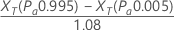
Minitab estimates the pre-adjusted repeatability by:

Notation
| Term | Description |
|---|---|
| XT | represents the estimated reference values at the 0.995 and 0.005 probabilities of acceptance, which are calculated from the fitted line on the probability plot. |
Repeatability
Repeatability is the amount of variation in the measurement system that is from the gage. An attribute gage study regresses the probabilities of acceptance on the reference values to obtain repeatability.
Pre-adjusted repeatability is the repeatability that is calculated before adjusting for over-estimation. Minitab divides estimates of repeatability by the adjustment factor 1.08 to calculate the adjusted repeatability.
Formula
Minitab estimates the repeatability by:
Notation
| Term | Description |
|---|---|
| XT | represents the estimated reference values at the 0.995 and 0.005 probabilities of acceptance, which are calculated from the fitted line on the probability plot. |
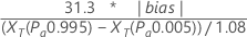
The denominator, 1.08, is the adjustment factor given by the Automotive Industry Action Group1 Minitab uses the adjusted repeatability value to test bias = 0.
T for the AIAG method
Formula
To test bias = 0 using the regression method, Minitab uses the following formula:
Notation
| Term | Description |
|---|---|
| XT | represents the estimated reference values at the 0.995 and 0.005 probabilities of acceptance, which are calculated from the fitted line on the probability plot. |
- 6 parts that have acceptances greater than 0 and less than 20
- 1 part has 0 acceptances
- 1 part has 20 acceptances
T for the regression method
Formula
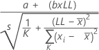
To test bias = 0 using the regression method, Minitab uses the following formula:
Notation
| Term | Description |
|---|---|
| a | the intercept of the probability plot's fitted line |
| b | the slope of the probability plot's fitted line |
| LL | lower tolerance limit |
| s | the error standard deviation calculated using the fitted line |
| K | the number of parts |
| xi | the reference value of each part |
 | the mean of the reference values |
DF for the AIAG method
The degrees of freedom is used to calculate the p-value.
DF = N – 1.
Notation
| Term | Description |
|---|---|
| N | number of trials |
DF for the regression method
The degrees of freedom is used to calculate the p-value.
DF = N – 2.
Notation
| Term | Description |
|---|---|
| N | number of points used to obtain the fitted line |
p-value
P-values are used in hypothesis tests to help you decide whether to reject or fail to reject a null hypothesis.
To determine whether bias in the measurement system is statistically significant, compare the p-value to the significance level. Usually, a significance level (denoted as α or alpha) of 0.05 works well. A significance level of 0.05 indicates a 5% risk of concluding that bias exists when there is no significant bias.
Fitted line
The fitted line is a regression line that examines the relationship between the probability of acceptances and the reference values of the measured parts.
The general form of a fitted line is: Y = b0 + b1 X
Minitab regresses the z–score Φ-1(Prob (Acceptance)) on reference values XT to get the intercept and slope.
Notation
| Term | Description |
|---|---|
| b0 | the intercept—the constant that determines the vertical placement of the regression line |
| b1 | the slope of the regression line |
| X | the predictor value |
R-sq for Fitted Line
R-sq for Fitted Line is the coefficient of determination, which is used to check whether the fitted line models the data well. The R-sq (R2) value for the fitted regression line indicates the percentage of the variation in the probability of acceptance responses that is explained by the regression model.
R2 = 1 - (SS error / SS total)
Notation
| Term | Description |
|---|---|
| SS error | sum of square for the error |
| SS total | total sum of squares |