ML estimates of distribution parameters
The Maximum Likelihood (ML) method estimates the values of the distribution parameters that maximize the likelihood function for each distribution. The goal is to obtain the best agreement between the distribution model and the observed sample data.
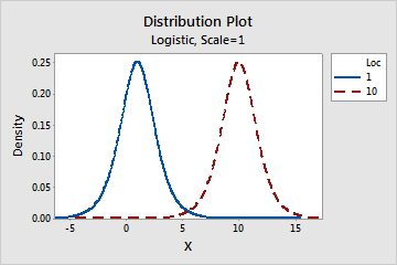
- Location
- This parameter affects the location of a distribution. For example, with different location
parameters, a logistic distribution can be shifted along the horizontal
axis.
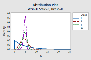
- Shape
- This parameter affects the shape of the distribution. For example, with different shape
parameters, a Weibull distribution can appear more skewed or more symmetric.
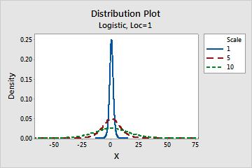
- Scale
- This parameter affects the scale of the distribution. For example, with different scale
parameters, a logistic distribution can appear more stretched out or more
compressed.
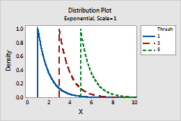
- Threshold
- This parameter affects the minimum value of a random variable. For example, with different
threshold parameters, an exponential distribution can be defined over a
different range of values.
Note
Minitab calculates the parameter estimates using maximum likelihood method for all the distributions except normal and lognormal distributions, which instead use unbiased parameter estimates.
Interpretation
Use the ML estimates of the distribution parameters to understand the specific distribution model that is used for your data. For example, suppose a quality engineer decides that, based on historical process knowledge and the Anderson-Darling and LRT p-values, the 3-parameter Weibull distribution provides the best fit for the process data. To understand the specific 3-parameter Weibull distribution that is used to model the data, the engineer examines the ML estimates for shape, scale, and threshold that are calculated for the distribution.
Distribution
The analysis provides goodness-of-fit statistics and distribution parameters for several commonly used distributions. Many of these distributions are versatile and can model a variety of continuous data, including data with positive values, negative values, and 0.
- Lognormal
- Exponential
- Weibull
- Gamma
- Loglogistic
Therefore, if your data contain negative values or 0, Minitab does not report results for these specific distributions. In that case, use the results for the higher-parameter version of each distribution. For example, if your data contain negative values, Minitab does not report results for the lognormal distribution. Instead, use the results for the 3-parameter lognormal distribution.
For more information on the distributions, go to Why is Weibull the default distribution for nonnormal capability analysis?.
Note
For information on the formulas that are used to calculate the PDF and CDF for each distribution, go to Methods and formulas for distributions in Individual Distribution Identification.
P
Note
No p-value for the AD test is available for the 3-parameter distributions, except for the Weibull distribution.
Interpretation
Use the p-value to assess the fit of the distribution.
- P ≤ α: The data do not follow the distribution (Reject H0)
- If the p-value is less than or equal to the significance level, the decision is to reject the null hypothesis and conclude that your data do not follow the distribution.
- P > α: Cannot conclude the data do not follow the distribution (Fail to reject H0)
- If the p-value is greater than the significance level, the decision is to fail to reject the null hypothesis. There is not enough evidence to conclude that the data do not follow the distribution. You can assume the data follow the distribution.
- Choose the distribution that is most commonly used in your industry or application.
- Choose the distribution that provides the most conservative results. For example, if you are performing capability analysis, you can perform the analysis using different distributions and then choose the distribution that produces the most conservative capability indices. For more information, go to Distribution percentiles for Individual Distribution Identification and click "Percents and percentiles".
- Choose the simplest distribution that fits your data well. For example, if a 2-parameter and a 3-parameter distribution both provide a good fit, you might choose the simpler 2-parameter distribution.
Important
Use caution when you interpret results from a very small or a very large sample. If you have a very small sample, a goodness-of-fit test may not have enough power to detect significant deviations from the distribution. If you have a very large sample, the test may be so powerful that it detects even small deviations from the distribution that have no practical significance. Use the probability plots in addition to the p-values to evaluate the distribution fit.
Automated Capability Distribution Results: Calcium
| Distribution | Location | Scale | Threshold | Shape | P | Ppk | Cpk |
|---|---|---|---|---|---|---|---|
| Normal | 50.7820 | 2.7648 | 0.0463827 | 1.2999 | 1.3504 | ||
| Weibull | 52.1368 | 17.825 | <0.01 | 0.7907 | |||
| Lognormal* | 3.9261 | 0.0537 | 0.0848247 | 1.4732 | |||
| Smallest Extreme Value | 52.2226 | 2.9589 | <0.01 | 0.7153 | |||
| Largest Extreme Value | 49.5037 | 2.1699 | >0.25 | ||||
| Gamma | 0.1447 | 351.044 | 0.0706812 | 1.4275 | |||
| Logistic | 50.5718 | 1.5948 | 0.0339831 | 1.0023 | |||
| Loglogistic | 3.9226 | 0.0312 | 0.0495201 | 1.0864 | |||
| Exponential | 50.7820 | <0.0025 | -0.0378 | ||||
| 3-Parameter Weibull | 4.5365 | 46.6658 | 1.476 | >0.5 | |||
| 3-Parameter Lognormal | 1.6930 | 0.4685 | 44.7401 | ||||
| 3-Parameter Gamma | 1.6370 | 45.8838 | 2.992 | ||||
| 3-Parameter Loglogistic | 1.5486 | 0.3276 | 45.4618 | ||||
| 2-Parameter Exponential | 4.0633 | 46.7187 | 0.0140796 | ||||
| Box-Cox transformation | 0.0000 | 0.0000 | 0.324445 | 2.5062 | 2.5335 | ||
| Johnson transformation | 0.0290 | 0.9729 | 0.985835 | 2.7129 | |||
| Nonparametric | 2.8889 |
In these results, the lognormal distribution is the first method that fits the data at the 0.05 significance level. Other distributions and transformations also provide an adequate fit to the data. Consider whether any of these alternate methods are more compatible with the process.
Note
For several distributions, Minitab also displays results for the distribution with an additional parameter. For example, for the lognormal distribution, Minitab displays results for both the 2-parameter and 3-parameter versions of the distribution. For distributions that have additional parameters, consider whether the additional parameter is compatible with what you know about the process. For example, if the process has a physical boundary at a non-zero value, then a distribution with a threshold parameter is compatible with the process.
Ppk
- The distance from the process mean to the closest specification limit (USL or LSL)
- The one-sided spread of the process (the 3-σ variation) based on its overall variation
Interpretation
Use Ppk to evaluate the overall capability of your process based on both the process location and the process spread. Overall capability indicates the actual performance of your process that your customer experiences over time.
Generally, higher Ppk values indicate a more capable process. Lower Ppk values indicate that your process may need improvement.
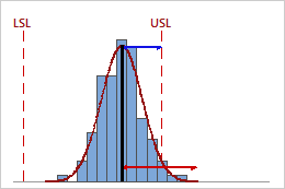
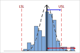
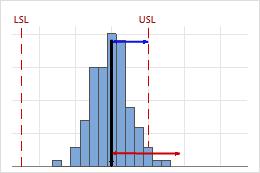
Low Ppk
In this example, the distance from the process mean to the nearest specification limit (USL) is less than the one-sided process spread. Therefore, Ppk is low (0.66), and the overall capability of the process is poor.
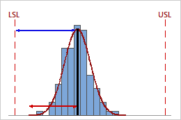
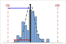
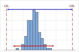
High Ppk
In this example, the distance from the process mean to the nearest specification limit (LSL) is greater than the one-sided process spread. Therefore, Ppk is high (1.68), and the overall capability of the process is good.
-
Compare Ppk to a benchmark value that represents the minimum value that is acceptable for your process. Many industries use a benchmark value of 1.33. If Ppk is lower than your benchmark, consider ways to improve your process.
-
Compare Pp and Ppk. If Pp and Ppk are approximately equal, then the process is centered between the specification limits. If Pp and Ppk differ, then the process is not centered.
-
Compare Ppk and Cpk. When a process is in statistical control, Ppk and Cpk are approximately equal. The difference between Ppk and Cpk represents the improvement in process capability that you could expect if shifts and drifts in the process were eliminated.
Caution
The Ppk index represents only one side of the process curve and does not measure how the process performs on the other side of the process curve.
For example, the following graphs display two processes that have identical Ppk values. However, one process violates both specification limits, and the other process violates only the upper specification limit.
Ppk = min {PPL = 4.01, PPU = 0.64} = 0.64
Ppk = PPL = PPU = 0.64
If your process has nonconforming parts that fall on both sides of the specification limits, consider using other indices, such as Z.bench, to more fully assess process capability.
Cpk
- The distance from the process mean to the closest specification limit (USL or LSL)
- The one-sided spread of the process (the 3-σ variation) based on the within-subgroup standard deviation
Interpretation
Use Cpk to evaluate the potential capability of your process based on both the process location and the process spread. Potential capability indicates the capability that could be achieved if process shifts and drifts were eliminated.
Generally, higher Cpk values indicate a more capable process. Lower Cpk values indicate that your process may need improvement.
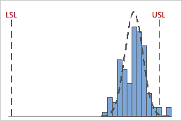
Low Cpk
In this example, the distance from the process mean to the nearest specification limit (USL) is less than the one-sided process spread. Therefore, Cpk is low (0.80), and the potential capability of the process is poor.
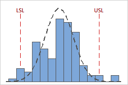
High Cpk
In this example, the distance from the process mean to the nearest specification limit (LSL) is greater than the one-sided process spread. Therefore, Cpk is high (1.64), and the potential capability of the process is good.
You can compare Cpk with other values to get more information about the capability of your process.
-
Compare Cpk with a benchmark that represents the minimum value that is acceptable for your process. Many industries use a benchmark value of 1.33. If Cpk is lower than your benchmark, consider ways to improve your process, such as reducing its variation or shifting its location.
-
Compare Cp and Cpk. If Cp and Cpk are approximately equal, then the process is centered between the specification limits. If Cp and Cpk differ, then the process is not centered.
-
Compare Ppk and Cpk. When a process is in statistical control, Ppk and Cpk are approximately equal. The difference between Ppk and Cpk represents the improvement in process capability that you could expect if shifts and drifts in the process were eliminated.
Caution
The Cpk index represents only one side of the process curve, and does not measure how the process performs on the other side of the process curve.
For example, the following graphs display two processes with identical Cpk values. However, one process violates both specification limits, and the other process only violates the upper specification limit.
Cpk = min {CPL = 4.58, CPU = 0.93} = 0.93
Cpk = CPL = CPU = 0.93
If your process has nonconforming parts that fall on both sides of the specification limits, consider using other indices to more fully assess process capability.
Cnpk
Cnpk is a measure of the overall capability of the process and equals the minimum of Cnpu and Cnpl.
- The one-sided specification spread, from the process median to the upper specification limit
- One-half the process spread, from the process median to the estimate of the upper end of the process
- The one-sided specification spread, from the process median to the lower specification limit
- One-half the process spread, from the process median to the estimate of the lower end of the process
Interpretation
Use Cnpk to evaluate the overall capability of your process based on both the process location and the process spread. Overall capability indicates the actual performance of your process that your customer experiences over time.
Generally, higher Cnpk values indicate a more capable process. Lower Cnpk values indicate that your process may need improvement.
Low Cnpk
In this example, the process is performing worse in relation to its upper specification limit than its lower specification limit. The Cnpk value equals Cnpu (≈ 0.40), which is low and indicates poor capability.
High Cnpk
In this example, the process is performing worse in relation to its lower specification limit than its upper specification limit. The Cnpk value equals Cnpl (≈ 1.40), which is high and indicates good capability.
-
If Cnpk < 1, then the specification spread is less than the process spread.
-
Compare Cnpk to a benchmark value that represents the minimum value that is acceptable for your process. Many industries use a benchmark value of 1.33. If Cnpk is lower than your benchmark, consider ways to improve your process.
CAUTION
The Cnpk index represents the process capability for only the "worse" side of the process measurements, that is, the side that exhibits poorer process performance. If your process has nonconforming parts that fall on both sides of the specification limits, check the capability graphs and the probabilities of parts outside both specification limits to more fully assess process capability.