Quality engineers at a company that manufactures floor tiles investigate customer complaints about warping in the tiles. To ensure production quality, the engineers measure warping in 10 tiles each working day for 10 days. The upper specification limit for the warping measurement is 6 mm. The engineers want to explore different options to find a reasonable method to estimate the capability of the process.
- Open the sample data, TileWarping.MWX.
- Choose .
- In Single column, enter Warping.
- In Subgroup size, enter 10.
- In Upper spec, enter 6.
- Select OK.
Interpret the results
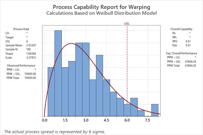
The analysis displays a capability report for the first method that provides a reasonable fit. For the warping of the tiles, the results use a Weibull distribution.
For these data, measurements on the right tail of the histogram appear to fall above the upper specification limit. Therefore, the warping of the tiles frequently exceeds the upper specification limit of 6 mm. The observed PPM > USL indicates that 70,000 out of every million tiles are above the upper specification limit. The overall Ppk is 0.51, which is less than the generally accepted industry guideline of 1.33. Therefore, the engineers conclude that the process is not capable and does not meet customer requirements.
The table of distribution results shows the order of the evaluation of the methods. In the first row, the conclusion for the Anderson-Darling test is that the data do not follow a normal distribution at the 0.05 level of significance because the p-value is less than 0.05. In the second row, the conclusion for the Anderson-Darling test is that the Weibull distribution is a reasonable fit to the data because the p-value is greater than 0.05. The capability results are for the Weibull distribution because the Weibull distribution is the first method in the list that provides a reasonable fit.
The engineers use process knowledge to consider whether the Weibull distribution is a reasonable selection. For example, the Weibull distribution has a boundary at 0. In the data, 0 is a boundary that represents an unwarped tile.
Automated Capability Distribution Results: Warping
| Distribution | Location | Scale | Threshold | Shape | P | Ppk | Cpk |
|---|---|---|---|---|---|---|---|
| Normal | 2.9231 | 1.7860 | 0.0100421 | 0.5743 | 0.5838 | ||
| Weibull* | 3.2781 | 1.6937 | >0.25 | 0.5133 | |||
| Lognormal | 0.8443 | 0.7444 | <0.005 | 0.4242 | |||
| Smallest Extreme Value | 3.8641 | 1.9924 | <0.01 | 0.5362 | |||
| Largest Extreme Value | 2.0958 | 1.4196 | 0.212835 | 0.5130 | |||
| Gamma | 1.2477 | 2.3428 | 0.238337 | 0.4851 | |||
| Logistic | 2.7959 | 1.0162 | 0.0127347 | 0.5799 | |||
| Loglogistic | 0.9097 | 0.4217 | <0.005 | 0.4090 | |||
| Exponential | 2.9231 | <0.0025 | 0.3780 | ||||
| 3-Parameter Weibull | 2.9969 | 0.2099 | 1.5049 | 0.467097 | 0.4980 | ||
| 3-Parameter Lognormal | 1.3788 | 0.4184 | -1.4002 | 0.4961 | |||
| 3-Parameter Gamma | 1.2314 | -0.0197 | 2.3898 | 0.4864 | |||
| 3-Parameter Loglogistic | 1.3043 | 0.2700 | -1.0940 | 0.4656 | |||
| 2-Parameter Exponential | 2.6679 | 0.2552 | <0.01 | 0.3982 | |||
| Box-Cox transformation | 1.6237 | 0.5380 | 0.574337 | 0.5116 | 0.5214 | ||
| Johnson transformation | 0.0112 | 0.9949 | 0.798895 | 0.4959 | |||
| Nonparametric | 0.6187 |