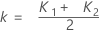
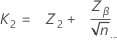
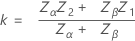
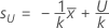
The calculation of sample size, n, and critical distance, k, depends on the number of specification limits given and whether standard deviation is known.
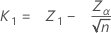
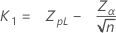
Single specification limit and known standard deviation
The sample size is given by:
The critical distance is given by:
where:
Notation
Term
Description
Z1
the (1 – p1) * 100 percentile of the standard normal distribution
p1
the Acceptable Quality Level (AQL)
Z2
the (1 – p2) * 100 percentile of the standard normal distribution
p2
the Rejectable Quality Level (RQL)
Zα
the (1 – α) * 100 percentile of the standard normal distribution
α
the producer's risk
Zβ
the (1 – β ) * 100 percentile of the standard normal distribution
β
the consumer's risk
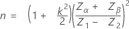
Single specification limit and unknown standard deviation
Notation is the same as for the section for a single specification limit and a known standard deviation. The sample size is given by:
The critical distance is given by:
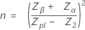
Double specification limits and known standard deviation
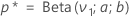
Notation not defined below is the same as for the case for a single specification limit and a known standard deviation. First Minitab calculates z:
Then Minitab finds p* from the standard normal distribution as the upper tail area corresponding to z. This is the minimum probability of defective outside one of the specification limits.
The method that Minitab uses for the calculation of the sample size and the critical distance depends on this value of p*.
Let p1 = AQL, p2 = RQL
If 2p* ≤ (p1/ 2), then the two specifications are relatively far apart and calculations follow the single limit plans.
If p1/ 2 < 2p* ≤ p1, then the two specifications are not relatively far apart, but are still not so close that the minimum probability of defective can be found for certain mean values. Minitab performs an iteration to find sample size and critical distance.
Let
μ = μ0+ m * h, where h = σ/100
Let m = 1, 2, ...300. For each μ calculate:
where Φ is the cumulative distribution function of the standard normal distribution. If Prob (X<L) + Prob (X>U) is extremely close to p1, then Minitab uses the larger value between Prob (X<L) and Prob (X>U) to find sample size and accept number.
Suppose Prob (X<L) is the larger value, let pL = Prob (X<L).
The sample size is given by:
The critical distance is given by:
where:
ZpL = the (1 – pL) * 100 percentile of the standard normal distribution.
If we already use all the m values but the corresponding probabilities do not contain p1, then p1 is too large, which means that the mean of the measurements is far away from the midpoint of the interval [L, U]. In this case, we can use a method for a single specification limit and ZpL = Z1. Z1 has the same definition as for the single specification limit case.
If p1 < 2p* < p2, then the specifications of the plan must be reconsidered because the minimum probability defective determined by the two specification limits and the standard deviations is larger than the acceptable quality level p1. You can reject the lot or consider a plan with a slightly larger probability of defective than p1.
If 2p* ≥ p2, then the lot should be rejected; the minimum probability of defective determined by the two specification limits and the standard deviation is larger than the rejectable quality level. You can reject the lot without testing any products.
Notation
Term
Description
L
the lower specification limit
U
the upper specification limit
σ
the known standard deviation
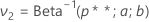
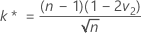
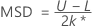
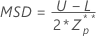
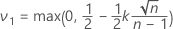
Double specification limits and unknown standard deviation (Default procedure)
Notation is the same as for the previous sections. Minitab lets the critical distance be the value as given in the case of two separate single-limit plans:
The sample size is given by:
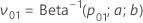
If n > 2, then Minitab calculates the MSD with the following steps1.
Let
Then,
where Beta is the cumulative distribution function of a beta distribution with shape parameters a and b. Here, .
Define
Then,
where Beta-1 is the inverse cumulative distribution function of the beta distribution from step 2.
If n ≤ 2, The Maximum Standard Deviation (MSD) is incalculable.
Double specification limits and unknown standard deviation (Wallis procedure)
Notation is the same as for the previous sections. The following procedure can be found in Schilling's book.2
First Minitab lets the critical distance be the value as given in the case of two separate single-limit plans:
Then Minitab finds the upper tail area from the standard normal distribution, p*, corresponding to the k as the percentile; and the percentile Zp** from the standard normal distribution corresponding to upper tail area of p* / 2.
The maximum standard deviation (MSD) is given by:
The estimated standard deviation is given by:
Minitab tests whether the estimated standard deviation, s, is less than or equal to the MSD.
If the estimated standard deviation, s, is less than or equal to the MSD, then the sample size is given by:
If the estimated standard deviation, s, is not less than or equal to the MSD, then the standard deviation is too large to be consistent with acceptance criteria and you must reject the lot.
Notation
Term
Description
Xi
the ith measurement
the mean of actual measurements
Probability of acceptance
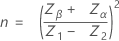
Let p be the probability of defective which is the x value of a point on an OC curve.
Single specification limit and known standard deviation
Single lower specification limit and known standard deviation
Prob (X < L) = p.
Single upper specification limit and known standard deviation
Prob (X > L) = p.
Single specification limit and unknown standard deviation
Double specification limits and known standard deviation
First Minitab calculates z
Then finds p* from the standard normal distribution as the upper tail area corresponding to z. This is the minimum probability of defective outside one of the specification limits.
The method Minitab uses for the probability of acceptance depends on this value of p*.
Let p1 = AQL, p2 = RQL
If 2p* ≤ (p1/ 2), then the two specifications are relatively far apart and calculations for sample size and critical distance follow the single limit plans.
If p1/ 2 < 2p* ≤ p1, then the two specifications are not relatively far apart, but are still not so close that the minimum probability of defective can be found for certain mean values.
For any given p, Minitab finds the mean, μ, of the measurements using a grid search algorithm. Then,
Double specification limits and unknown standard deviation
When you have both upper and lower specification limits, but do not know the standard deviation, Minitab uses the OC curve for the single-limit plan to approximate the double specification limits case. The OC curve derived for a single-limit plan with specified p1, p2, α, and β is the lower limit of the band of OC curves for a two-sided specification plan with the same p1, p2, α, and β and for most practical cases can be taken as the OC curve for the two-sided plan. See Duncan1.
Duncan (1986). Quality Control and Industrial Statistics, 5th edition.
Notation
Term
Description
n
sample size
k
critical distance
σ
known standard deviation
Zp
the (1 - p)th percentile from the standard normal distribution
Φ
the cumulative distribution function of the standard normal distribution
T
is non-central t distributed with degrees of freedom = n – 1, and the non central parameter,
L
lower specification limit
U
upper specification limit
Probability of rejecting
The probability of rejecting (Pr) describes the chance of rejecting a particular lot based on a specific sampling plan and incoming proportion defective. It is simply 1 minus the probability of acceptance.
Pr = 1 – Pa
where:
Pa = probability of acceptance
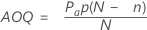
Average outgoing quality (AOQ)
The average outgoing quality represents the quality level of the product after inspection. The average outgoing quality varies as the incoming fraction defective varies.
Notation
Term
Description
Pa
probability of acceptance
p
incoming fraction defective
N
lot size
n
sample size
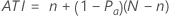
Average total inspection (ATI)
The average total inspection represents the average number of units that will be inspected for a particular incoming quality level and probability of acceptance.
Notation
Term
Description
Pa
probability of acceptance
N
lot size
n
sample size
Acceptance region (AR) - Default procedure
The acceptance region is calculated only when both specifications are given
and the standard deviation is unknown. Go to the section on sample size and
critical distance to find definitions for
n and
k, respectively, and to see the notation for the equations..
On the acceptance region plot, the x-axis is the sample mean and the y-axis
is the sample standard deviation. The acceptance region is formed by 3
functions of the sample standard deviation and the sample mean in addition to
the Maximum Standard Deviation (MSD). For any values of the sample mean where
the values of the sample standard deviation exceeds the MSD, the upper bound of
the acceptance region is the MSD.
For cases that are near the upper or lower specification limits, the
acceptance region is bounded by these two functions:
As the values of the sample mean get closer to the middle of the
specification limits, the coordinates of the upper boundary of the acceptance
region are calculated with the following steps:
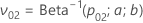
Let .
Then
where Beta is the cumulative distribution function of a beta distribution with
shape parameters
a and
b. Here, .
Define pairs of proportions
p01 and p02, that satisfy p02 + p01
= p*
Next,
where
Beta-1 is the inverse cumulative distribution function of the beta
distribution from step 2.
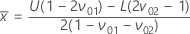
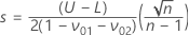
For ,
the mean and standard deviation coordinates are the following equations:
Acceptance region (AR) - Wallis procedure
The following calculations are for the case when the analysis has both
specifications but the standard deviation is unknown. The procedure can be
found in Schilling's book.2
In this plot, the x-axis shows values of the sample mean
()
and the y-axis shows values of the standard deviation. In combination with the
x-axis, the following lines form an acceptance triangle.
The dashed line and the x-axis form a more accurate region. Use the
following steps to form the dashed line.
Let p* be the upper tail area
from the standard normal distribution with the critical distance as the
percentile: P(Z > k).
Select values of
p01 and p02 that satisfy p02 + p01
= p*:
p01 = (p* /
100) * h
p02 = (p* /
100) * (100 - h)
where h takes the values 1 to 00.
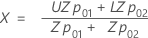
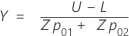
Use the following equations
to define the X and Y coordinates:
Notation
Term
Description
L
lower specification limit
U
upper specification limit
k
critical distance
Zp01
the (1 - p01)* 100 percentile from the
standard normal distribution
Zp02
the (1 - p02)* 100 percentile from the standard normal
distribution
p01
(p* / 100) *
h
p02
(p* / 100) * (100 –
h)
1 Duncan, A. J. (1986). Quality Control and Industrial Statistics (5th ed.). Homewood, Ill: Irwin.
2 Schilling and Neubauer (2009). Acceptance Sampling in Quailty Control (2nd ed.)


 .
. 


 .
.
 where Beta is the cumulative distribution function of a beta distribution with
shape parameters
a and
b. Here,
where Beta is the cumulative distribution function of a beta distribution with
shape parameters
a and
b. Here,  .
.
 ,
the mean and standard deviation coordinates are the following equations:
,
the mean and standard deviation coordinates are the following equations:
 )
and the y-axis shows values of the standard deviation. In combination with the
x-axis, the following lines form an acceptance triangle.
)
and the y-axis shows values of the standard deviation. In combination with the
x-axis, the following lines form an acceptance triangle.