In This Topic
Measurement type
- Defect
- A defect is a fault in a single item, such as a stain on a shirt. An item can have more than one defect.
- Defective
- A defective is a nonconforming item, such as a pen that does not work. An item is either defective or not defective.
Lot quality
The lot quality units of measure for an attributes acceptance sampling plan depend on whether you choose to count defective items or defects.
- Percent defective
- Represents the percentage defective as a value between 0 and 100. For example, if 10 units are defective out of a sample size of 500, the percent defective is 2.
- Proportion defective
- Represents the proportion defective as a value between 0 and 1. For example, if 10 units are defective out of a sample size of 500, the proportion defective is 0.02.
- Defectives per million
- Represents the level of defectives as a value out of a million units. For example, 10 defectives per million (DPM) means that you have 10 defective units for every million units.
- Defects per unit
- Defects per unit (DPU) is the average number of defects per unit observed when sampling a population.
- Defects per hundred
- Defects per hundred (DPH) is the average number of defects per hundred units observed when sampling a population.
- Defects per million
- Defects per million (DPM) is the average number of defects per million units observed when sampling a population.
Lot size
The lot size is the population that you collect your samples from when you decide whether to accept or reject the entire lot.
Often, the lot size is chosen to be convenient for shipping and handling for both the supplier and consumers. For example, a convenient lot size might be an entire shipment. Because sampling plans assume homogeneity of parts in a lot, the units that comprise a lot should be produced under the same process conditions. Also, larger lots are generally more economical to inspect than a series of smaller lots.
Acceptable Quality Level (AQL) and Rejectable Quality Level (RQL or LTPD)
- Acceptable quality level (AQL)
- The acceptable quality level (AQL) is the highest defective rate or defect rate from a supplier's process that is considered acceptable. The AQL describes what the sampling plan will accept, and the RQL describes what the sampling plan will reject. You want to design a sampling plan that accepts a particular lot of product at the AQL most of the time.
- Rejectable quality level (RQL or LTPD)
- The rejectable quality level (RQL) is the highest defective rate or defect rate that the consumer is willing to tolerate in an individual lot. The RQL describes what the sampling plan will reject, and the AQL describes what the sampling plan will accept. You want to design a sampling plan that rejects a particular lot of product at the RQL most of the time.
Interpretation
The consumer and supplier should agree to the highest defective rate or defect rate that is acceptable (AQL). The consumer and supplier should also agree to the highest defective rate or defect rate that the consumer will tolerate in an individual lot (RQL).
The probability of acceptance at the AQL (1.5% defective) is 0.95, and the probability of rejecting is 0.05. The probability of accepting at the RQL (10% defective) is 0.10, and the probability of rejecting is 0.90.
Method
| Acceptable Quality Level (AQL) | 1.5 |
|---|---|
| Producer’s Risk (α) | 0.05 |
| Rejectable Quality Level (RQL or LTPD) | 10 |
| Consumer’s Risk (β) | 0.1 |
Producer's risk (Alpha) and consumer's risk (Beta)
- Producer’s risk (Alpha)
- The producer's risk, α, is the probability of rejecting a lot that has a quality level equal to the AQL that should be accepted. As α increases, the risk of rejecting lots with defective rates equal to the AQL increases, which causes harm to the producer. The producer's risk is also known as type I error.
- Consumer’s risk (Beta)
- The consumer's risk, β, is the probability of accepting a lot with a quality level equal to the RQL that should be rejected. As β increases, the risk of accepting lots with defective rates equal to the RQL increases, which causes harm to the consumer. The consumer's risk is also known as type II error.
Interpretation
To protect the producer, the risk of rejecting a lot that has acceptable quality must be low. To protect the consumer, the risk of accepting a lot that has poor quality must be low.
The probability of acceptance at the AQL is 0.95, and the probability of rejecting is 0.05. The probability of accepting at the RQL is 0.10, and the probability of rejecting is 0.90.
Method
| Acceptable Quality Level (AQL) | 1.5 |
|---|---|
| Producer’s Risk (α) | 0.05 |
| Rejectable Quality Level (RQL or LTPD) | 10 |
| Consumer’s Risk (β) | 0.1 |
Sample size
In acceptance sampling, the sample size is the number of items that are randomly chosen from a single lot for inspection.
Interpretation
In this example, the sample size is 52. You must sample 52 items from the entire lot of product.
Generated Plan(s)
| Sample Size | 52 |
|---|---|
| Acceptance Number | 2 |
| Percent Defective | Probability Accepting | Probability Rejecting | AOQ | ATI |
|---|---|---|---|---|
| 1.5 | 0.957 | 0.043 | 1.420 | 266.2 |
| 10.0 | 0.097 | 0.903 | 0.956 | 4521.9 |
Acceptance number
The acceptance number is the maximum number of defects or defectives that are allowed in a sample from an acceptable lot.
Interpretation
In this example, the acceptance number is 2. You must sample 52 items from the entire lot of product. If 2 or less defective items are found, you accept the entire lot. If 3 or more defective items are found, you reject the entire lot.
Generated Plan(s)
| Sample Size | 52 |
|---|---|
| Acceptance Number | 2 |
| Percent Defective | Probability Accepting | Probability Rejecting | AOQ | ATI |
|---|---|---|---|---|
| 1.5 | 0.957 | 0.043 | 1.420 | 266.2 |
| 10.0 | 0.097 | 0.903 | 0.956 | 4521.9 |
Probability accepting and probability rejecting
The probability of accepting lots at the AQL should be close to 1 – α. The probability of accepting lots at the RQL should be close to β. The probability of rejecting is 1 – the probability of accepting.
Interpretation
The probability of acceptance at the AQL (1.5% defective) is 0.957, and the probability of rejecting is 0.043. The probability of accepting at the RQL (10.0% defective) is 0.097, and the probability of rejecting is 0.903.
Generated Plan(s)
| Sample Size | 52 |
|---|---|
| Acceptance Number | 2 |
| Percent Defective | Probability Accepting | Probability Rejecting | AOQ | ATI |
|---|---|---|---|---|
| 1.5 | 0.957 | 0.043 | 1.420 | 266.2 |
| 10.0 | 0.097 | 0.903 | 0.956 | 4521.9 |
AOQ and AOQL
The average outgoing quality level represents the relationship between the quality of the incoming material and the quality of the outgoing material, assuming that rejected lots will be 100% inspected and all defective items will be replaced or reworked.
Note
You must specify the lot size in order to calculate the AOQ and AOQL.
Interpretation
In this example, when the average incoming quality level is 1.5% defective, the average outgoing quality is 1.42% defective. When the average incoming quality level is 10.0% defective, the average outgoing quality is 0.956% defective. The incoming quality is worse than the outgoing quality because rejected lots will be 100% inspected and will have all nonconforming units replaced or reworked.
The worst average outgoing defect level (AOQL) of 2.603% defective occurs when the incoming quality level is 4.3% defective.
Method
| Acceptable Quality Level (AQL) | 1.5 |
|---|---|
| Producer’s Risk (α) | 0.05 |
| Rejectable Quality Level (RQL or LTPD) | 10 |
| Consumer’s Risk (β) | 0.1 |
Generated Plan(s)
| Sample Size | 52 |
|---|---|
| Acceptance Number | 2 |
| Percent Defective | Probability Accepting | Probability Rejecting | AOQ | ATI |
|---|---|---|---|---|
| 1.5 | 0.957 | 0.043 | 1.420 | 266.2 |
| 10.0 | 0.097 | 0.903 | 0.956 | 4521.9 |
Average Outgoing Quality Limit(s) (AOQL)
| AOQL | At Percent Defective |
|---|---|
| 2.603 | 4.300 |
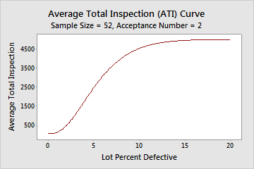
ATI
Note
You must specify the lot size in order to calculate the ATI.
Interpretation
In this example, when the average incoming quality level is 1.5% defective, the average number of units inspected per lot is 266.2. This is because 95.7% of the time you will inspect 52 items and pass the lot, and 4.3% of the time you will reject the lot and inspect all 5000 items. When the average incoming quality level is 10.0% defective, the average number of units inspected per lot is 4521.9, which is almost the entire shipment.
Generated Plan(s)
| Sample Size | 52 |
|---|---|
| Acceptance Number | 2 |
| Percent Defective | Probability Accepting | Probability Rejecting | AOQ | ATI |
|---|---|---|---|---|
| 1.5 | 0.957 | 0.043 | 1.420 | 266.2 |
| 10.0 | 0.097 | 0.903 | 0.956 | 4521.9 |
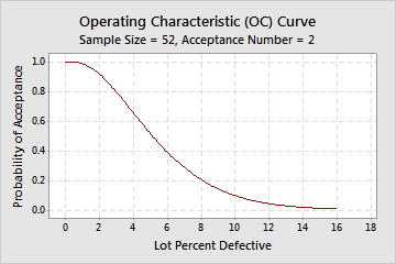
OC curve
The operating characteristic (OC) curve shows the ability of an acceptance sampling plan to distinguish between good and bad quality lots. The OC curve plots the probability of accepting lots that have different incoming quality levels for each sampling plan.
Interpretation
In this example, if the actual % defective is 1.5%, you have a 0.957 probability of accepting this lot based on the sample and a 0.043 probability of rejecting it. If the actual % defective is 10%, you have a 0.097 probability of accepting this lot and a 0.903 probability of rejecting it.
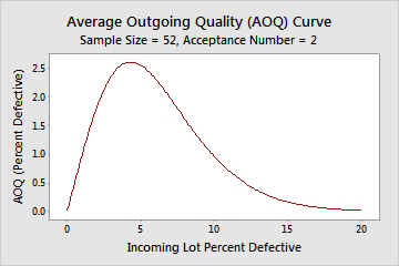
AOQ curve
Note
You must specify the lot size in order to create an AOQ curve.
Interpretation
In this example, when the average incoming quality level is 1.5% defective, the average outgoing quality is 1.42% defective. When the average incoming quality level is 10.0% defective, the average outgoing quality is 0.956% defective. The incoming quality is worse than the outgoing quality because rejected lots will be 100% inspected and will have all nonconforming units replaced or reworked.
The worst average outgoing defect level (AOQL) of 2.603% defective occurs when the incoming quality level is 4.3% defective.
ATI curve
Note
You must specify the lot size in order to create an ATI curve.
Interpretation